Introduction to Flux Balance Analysis Keesha Erickson - PowerPoint PPT Presentation
Introduction to Flux Balance Analysis Keesha Erickson keeshae@lanl.gov qBio Summer School June 21, 2018 Escherichia coli metabolic network Metabolism : the set of all biochemical reactions inside a cell Most metabolic reactions are catalyzed
Introduction to Flux Balance Analysis Keesha Erickson keeshae@lanl.gov qBio Summer School June 21, 2018
Escherichia coli metabolic network Metabolism : the set of all biochemical reactions inside a cell Most metabolic reactions are catalyzed by enzymes. Main functions of metabolism: ▪ Conversion of food/fuel to energy (ATP) ▪ Conversion of food/fuel to proteins, lipids, nucleic acids, etc ▪ Elimination of wastes From the Kyoto Encycolopedia of Genes and Genomes, http://www.genome.jp/kegg/
Metabolism provides important insights Studying evolution – Effects of horizontal gene transfer – Effects of gene deletion Prediction of essential genes – Minimal genome Metabolic engineering – Optimal overproduction of metabolites – Production coupled to growth Orth, Fleming, Palsson (2010) EcoSal Plus. Keasling. (2010) Science.
Flux Balance Analysis FBA can be used to calculate the flow of metabolites through a metabolic network FBA calculates rates ▪ Growth rate of an organism ▪ Production rate of a metabolite ▪ Yield of a product (production rate of product / consumption rate of substrate) Typical FBA does not: ▪ Use kinetic parameters, so cannot predict metabolite concentrations or estimate changes over time ▪ Consider regulatory effects (gene expression, enzyme cascades, etc) Orth et al. (2010) Nature Biotech.
Outline Metabolic network models ▪ Accounting for growth requirements ▪ Obtaining fluxes ▪ Tools for FBA ▪
Metabolic Network Models
Building a genome-scale metabolic network model Orth, Fleming, Palsson (2010) EcoSal Plus.
Reactions are associated with specific genes Gene: pgk Protein: Pgk (Phosphoglycerate kinase) Description: In glycolysis, catalyzes the transfer of a phosphoryl group from 1,3-bisphospho-D-glycerate to ADP, forming ATP and 3-phospho-D-glycerate Reaction: 13dpg[c] + adp[c] <=> 3pg[c] + atp[c] 13dpg 3pg PGK adp atp
Sets of reactions can be assembled into subsystems Orth, Fleming, Palsson (2010) EcoSal Plus.
Metabolic network models E. coli iJO1366: - 2251 metabolic reactions - 1136 unique metabolites Orth, Fleming, Palsson (2010) EcoSal Plus. Orth et al (2011) Mol Syst Biol.
BioModels Database 1990: first metabolic network model for E. coli (Majewski and Domach) 14 metabolic reactions 1997 : E. coli genome sequenced 2000: first genome-scale network model for E. coli (Edwards & Palsson) ~ 720 metabolic reactions 2003 : human genome sequenced 2007: first two metabolic network models for humans were published by Palsson group and Goryanin group ~ 3000 metabolic reactions 2011: E. coli model iJO1366 published (Orth et al) ~2000 metabolic reactions 2018: Rencon3D model of human metabolism published by Palsson group ~13000 metabolic reactions https://www.ebi.ac.uk/biomodels-main/ Accessed May 23, 2018
Metabolites Required attributes Name Description Charged Formula Charge Compartment
Reactions Required attributes Protein(s) Name Cellular subsystem Description Flux upper and lower bounds Formula Gene-reaction association Gene(s)
Accounting for growth requirements
The Biomass Reaction To predict growth rate, we need to estimate the rate at which metabolites are converted to biomass constituents (e.g., nucleic acids, proteins, lipids) The “biomass reaction” predicts the exponential growth rate (μ) of the organism. Coefficients on metabolites are experimentally determined. Biomass reaction for E. coli iJO1366: 0.000223 10fthf[c] + 0.000223 2dmmql8[c] + 2.5e-005 2fe2s[c] + 0.000248 4fe4s[c] + 0.000223 5mthf[c] + 0.000279 accoa[c] + 0.000223 adocbl[c] + 0.49915 ala-L[c] + 0.000223 amet[c] + 0.28742 arg-L[c] + 0.23423 asn-L[c] + 0.23423 asp-L[c] + 54.12 atp[c] + 0.000116 bmocogdp[c] + 2e-006 btn[c] + 0.004952 ca2[c] + 0.000223 chor[c] + 0.004952 cl[c] + 0.000168 coa[c] + 2.4e-005 cobalt2[c] + 0.1298 ctp[c] + 0.000674 cu2[c] + 0.088988 cys-L[c] + 0.024805 datp[c] + 0.025612 dctp[c] + 0.025612 dgtp[c] + 0.024805 dttp[c] + 0.000223 enter[c] + 0.000223 fad[c] + 0.006388 fe2[c] + 0.007428 fe3[c] + 0.25571 gln-L[c] + 0.25571 glu-L[c] + 0.5953 gly[c] + 0.15419 glycogen[c] + 0.000223 gthrd[c] + 0.20912 gtp[c] + 48.7529 h2o[c] + 0.000223 hemeO[c] + 0.092056 his-L[c] + 0.28231 ile-L[c] + 0.18569 k[c] + 0.43778 leu-L[c] + 3e-006 lipopb[c] + 0.33345 lys-L[c] + 3.1e-005 malcoa[c] + 0.14934 met-L[c] + 0.008253 mg2[c] + 0.000223 mlthf[c] + 0.000658 mn2[c] + 7e-006 mobd[c] + 7e-006 mococdp[c] + 7e-006 mocogdp[c] + 0.000223 mql8[c] + 0.001787 nad[c] + 4.5e-005 nadh[c] + 0.000112 nadp[c] + 0.000335 nadph[c] + 0.012379 nh4[c] + 0.000307 ni2[c] + 0.012366 pe160[c] + 0.009618 pe161[c] + 0.004957 pe181[c] + 0.005707 pg160[c] + 0.004439 pg161[c] + 0.002288 pg181[c] + 0.18002 phe-L[c] + 0.000223 pheme[c] + 0.2148 pro-L[c] + 0.03327 ptrc[c] + 0.000223 pydx5p[c] + 0.000223 q8h2[c] + 0.000223 ribflv[c] + 0.20968 ser-L[c] + 0.000223 sheme[c] + 0.004126 so4[c] + 0.006744 spmd[c] + 9.8e-005 succoa[c] + 0.000223 thf[c] + 0.000223 thmpp[c] + 0.24651 thr-L[c] + 0.055234 trp-L[c] + 0.13399 tyr-L[c] + 5.5e-005 udcpdp[c] + 0.1401 utp[c] + 0.41118 val-L[c] + 0.000324 zn2[c] + 0.008151 colipa[e] + 0.002944 clpn160[p] + .00229 clpn161[p] + 0.00118 clpn181[p] + 0.001345 murein3p3p[p] + 0.000605 murein3px4p[p] + 0.005381 murein4p4p[p] + 0.005448 murein4px4p[p] + 0.000673 murein4px4px4p[p] + 0.031798 pe160[p] + 0.024732 pe161[p] + 0.012747 pe181[p] + 0.004892 pg160[p] + 0.003805 pg161[p] + 0.001961 pg181[p] -> 53.95 adp[c] + 53.95 h[c] + 53.9459 pi[c] + 0.74983 ppi[c]
Energy requirements There are two reactions that account for energy required to maintain viability Growth associated maintenance (GAM) represents ATP needed for replication. It is included as part of the biomass reaction. Non-growth associated maintenance (NGAM) accounts for all other energy needs, and the constraint on this reaction is experimentally determined. atp[c] + h2o[c] -> adp[c] + h[c] + pi[c] (Lower bound of 3.15 mmol/gdcw/hr in iJO1366) Thiele & Palsson (2010) Nature Protocols.
FBA: Calculating fluxes for all reactions in the network, given an objective and constraints
Stoichiometric matrix S matrix: Reactions in columns Rows are metabolites Negative indicates consumption (reactant) Positive indicates production (product) Becker et al (2007) Nature Protocols.
Exercise 1 Write the S for the following system: Reactions Ex_glc glc <=> 0 Ex_o2 o2 <=> 0 R1 glc -> A glc R2 A <=> C A C Ex_glc R1 R2 R3 R3 C -> 0 R4 A + o2 <=> B R5 B -> 0 Ex_o2 R4 o2 -1 0 -1 0 0 0 0 glc B 0 -1 0 0 0 -1 0 o2 S = 0 0 1 -1 0 -1 0 A R5 0 0 0 0 0 1 -1 B 0 0 0 1 -1 0 0 C
The steady state assumption The inner product of the stoichiometric matrix S (size m x r) and the flux vector v (length r) gives the change in metabolite concentrations over time (d x /dt), where x is a vector of metabolite concentrations (length m). We are interested in solving for v . Assuming the cell is in one phenotype for a time longer than it takes for metabolite concentrations to change dramatically, we make the steady state assumption: Now we can solve for v . However, as there are many more reactions (unknown variables) than metabolites, there will not be one unique solution. Thus, it is helpful to impose constraints.
Constraining the solution space Orth & Thiele (2010) Nature Biotech. Becker et al (2007) Nature Protocols.
The linear programming problem Linear programming : optimizing a linear function subject to various constraints Canonical form: maximize c T x subject to A x ≤ b Flux Stoichiometric matrix Constraints and x ≥ 0 weighing Columns: reactions on flux vector Rows: metabolites Determine x given A and b For FBA: Metabolite Flux vector maximize c T v concentration (unknown) changes subject to S v = 0 and lb ≤ v ≤ ub Determine v given S and lb , ub
Exercise 2 Write S , c , lb , and ub for the following system, where you want to maximize production of species C. Reactions Ex_glc glc <=> 0 Ex_o2 o2 <=> 0 R1 glc -> A glc A C R1 R2 Ex_glc R3 R2 A <=> C R3 C -> 0 R4 A + o2 <=> B Ex_o2 R5 B -> 0 R4 o2 B R5
Exercise 2 Reactions glc Ex_glc glc <=> 0 A C R2 Ex_glc R1 R3 Ex_o2 o2 <=> 0 R1 glc -> A R2 A <=> C Ex_o2 R3 C -> 0 R4 R4 A + o2 <=> B o2 R5 B -> 0 B R5 0 -1000 1000 0 -1000 1000 -1 0 -1 0 0 0 0 glc 1000 0 0 0 -1 0 0 0 -1 0 o2 c = 0 -1000 ub = 1000 lb = S = 0 0 1 -1 0 -1 0 A 1 0 1000 0 0 0 0 0 1 -1 B 0 -1000 1000 0 0 0 1 -1 0 0 C 1000 0 0
Important constraints Reversibility Substrates/media conditions ▪ Carbon source ▪ Nitrogen source Varma & Palsson (1994) Applied Environmental Biology: Growth conditions ▪ Anaerobic ▪ Aerobic Minimum growth rate
Selecting the objective What do you want to maximize/minimize? Common objectives: Objective Rationale Example reaction Biomass reaction Biologically relevant – biomass safe to assume organism tries to optimize growth Transport reaction Calculate maximum EX_etoh(e) theoretical yield or production rate
Recommend
More recommend
Explore More Topics
Stay informed with curated content and fresh updates.

