Introduction to Bayesian Statistics Lecture 3: Single Parameter (II) - PowerPoint PPT Presentation

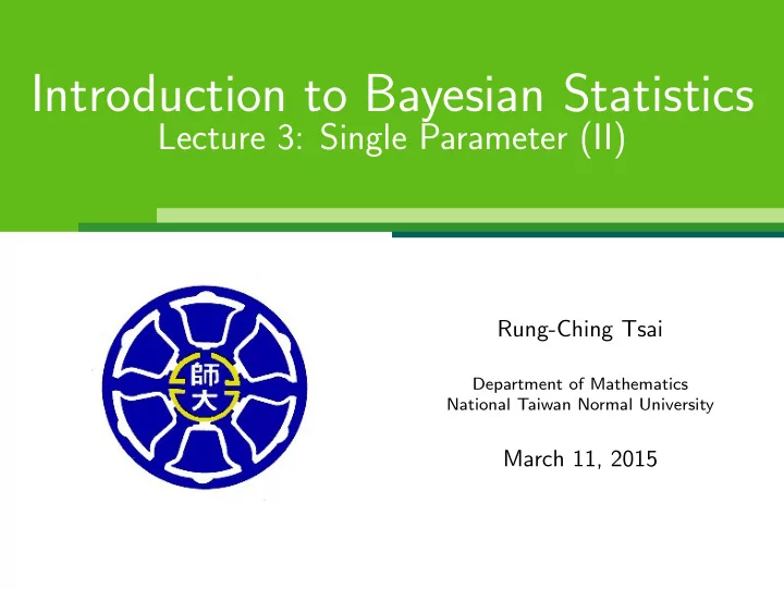
Introduction to Bayesian Statistics Lecture 3: Single Parameter (II) Rung-Ching Tsai Department of Mathematics National Taiwan Normal University March 11, 2015

Conjugate Prior Distributions Definition of Conjugacy: If F is a class of sampling distributions p ( y | θ ), and P is a class of prior distributions for θ , then the class P is conjugate for F if p ( θ | y ) ∈ P for all p ( ·| θ ) ∈ F and p ( θ ) ∈ P . • Advantages of using conjugate priors: ◦ computational convenience ◦ being interpretable as additional data • Example: Beta is conjugate for binomial with θ ∼ Beta( α, β ) and θ | y ∼ Beta( α + y , β + n − y ). • Exercise: What is the conjugate prior for Poisson( λ )? 2 of 14

Conjugate Prior Distributions for exponential families Definition: The class F is an exponential family if all its members have the form p ( y i | θ ) = f ( y i ) g ( θ )e φ ( θ ) T u ( y i ) , where φ ( θ ): the “natural parameter” of the family F . Exercise: Show that the binomial( n , θ ) is an exponential family with natural parameter logit( θ ), and the conjugate prior on θ are Beta distributions. 3 of 14

Conjugate Prior Distributions for exponential families • Likelihood of θ : � n n � � � � g ( θ ) n exp φ ( θ ) T � p ( y | θ ) = f ( y i ) u ( y i )) i =1 i =1 � � g ( θ ) n exp φ ( θ ) T t ( y ) ∝ , where t ( y ) = � n i =1 u ( y i ): sufficient statistic for θ • (Conjugate) Prior: � � p ( θ ) ∝ g ( θ ) η exp φ ( θ ) T ν • Posterior: � � p ( θ | y ) ∝ g ( θ ) η + n exp φ ( θ ) T ( ν + t ( y ) . • Known fact: Exponential families are, in general, the only classes of distributions that have natural conjugate priors. 4 of 14

Single Parameter θ : Continuous y • y ∼ normal( θ, σ 2 ), σ 2 known, use Bayesian approach to estimate θ . ◦ choose a conjugate prior for θ , p ( θ ) = e A θ 2 + B θ + C , such that � � − 1 ( θ − µ 0 ) 2 p ( θ ) ∝ exp 2 τ 2 0 1 � − 1 2 σ 2 ( y − θ ) 2 � ◦ likelihood of θ : p ( y | θ ) = 2 πσ exp √ ◦ find the posterior distribution of θ : � ( y − θ ) 2 + ( θ − µ 0 ) 2 � − 1 �� p ( θ | y ) ∝ p ( θ ) p ( y | θ ) ∝ exp τ 2 2 σ 2 0 � − 1 � ( θ − µ 1 ) 2 ∝ exp , 2 τ 2 1 that is, θ | y ∼ normal( µ 1 , τ 2 1 ), where 1 µ 0 + 1 σ 2 y τ 2 1 1 0 + 1 µ 1 = and 1 = 0 σ 2 . 1 + 1 τ 2 τ 2 τ 2 σ 2 0 5 of 14

Single Parameter θ : Continuous y • θ ∼ normal( µ 0 , τ 2 0 ) , y ∼ normal( θ, σ 2 ) ⇒ θ | y ∼ normal( µ 1 , τ 2 1 ) 1 • posterior precision τ 2 1 ◦ Definition of precision: the inverse of variance 1 1 0 + 1 ◦ 1 = σ 2 , i.e., the posterior precision equals the prior precision τ 2 τ 2 plus the data precision. • posterior mean µ 1 1 µ 0 + 1 σ 2 y τ 2 ◦ µ 1 = , i.e., the posterior mean is a weighted average of the 0 1 + 1 τ 2 σ 2 0 prior mean and the observed value y , with weights proportional to the precision. ◦ the prior mean adjusted toward the observed y : τ 2 µ 1 = µ 0 + ( y − µ 0 ) 0 0 . σ 2 + τ 2 ◦ a compromise between the prior mean and the observed data y , with σ 2 data shrunk toward the prior mean: µ 1 = y − ( y − µ 0 ) σ 2 + τ 2 0 6 of 14

Single Parameter θ : Continuous y Posterior predictive distribution p (˜ y | y ) � p (˜ y | y ) = p (˜ y | θ ) p ( θ | y ) d θ � � � � � − 1 − 1 y − θ ) 2 ( θ − µ 1 ) 2 ∝ exp 2 σ 2 (˜ exp d θ 2 τ 2 1 • ˜ y | y ∼ normal(? , ?) • E(˜ y | y ) = E(E(˜ y | θ, y ) | y ) = E( θ | y ) = µ 1 • var(˜ y | y ) = E(var(˜ y | θ, y ) | y ) + var(E(˜ y | θ, y ) | y ) = E( σ 2 | y ) + var( θ | y ) = σ 2 + τ 2 1 . y | θ ) = σ 2 Note. E(˜ y | θ ) = θ , var(˜ 7 of 14

Single Parameter θ : Continuous y = ( y 1 , · · · , y n ) iid ∼ normal( θ, σ 2 ), σ 2 known, use Bayesian approach to • y 1 , · · · , y n estimate θ . � 0 ( θ − µ 0 ) 2 � − 1 ◦ choose a conjugate prior for θ , p ( θ ) ∝ exp 2 τ 2 ◦ likelihood of θ : p ( y | θ ) = � n 1 � − 1 2 σ 2 ( y i − θ ) 2 � 2 πσ exp i =1 √ ◦ find the posterior distribution of θ : �� n i =1 ( y i − θ ) 2 + ( θ − µ 0 ) 2 � − 1 �� p ( θ | y ) ∝ p ( θ ) p ( y | θ ) ∝ exp τ 2 2 σ 2 0 � − 1 � ( θ − µ n ) 2 ∝ exp , 2 τ 2 n that is, θ | y ∼ normal( µ n , τ 2 n ), where 1 µ 0 + n σ 2 ¯ y τ 2 1 1 0 + n µ n = and n = σ 2 . 0 1 + n τ 2 τ 2 τ 2 σ 2 0 8 of 14

Single Parameter θ : Continuous y = ( y 1 , · · · , y n ) ∼ normal( θ, σ 2 ), σ 2 known, θ ∼ normal( µ 0 , τ 2 iid • y 1 , · · · , y n 0 ) ⇒ θ | y ∼ normal( µ n , τ 2 n ) 1 µ 0 + n σ 2 ¯ y τ 2 1 n = 1 0 + n • posterior precision σ 2 ; posterior mean µ n = 0 τ 2 τ 2 1 + n τ 2 σ 2 0 ◦ If n is large, the posterior distribution is largely determined by σ 2 and the sample value ¯ y . ◦ As τ 0 → ∞ with n fixed, or as n → ∞ with τ 2 0 fixed, we have y , σ 2 p ( θ | y ) ≈ normal( θ | ¯ n ) . ◦ Compare the well-known result of classical statistics: y | θ, σ 2 ∼ normal( θ, σ 2 y ± 1 . 96 σ ¯ n ) leads to the use of ¯ √ n as a 95% confidence interval for θ . ◦ Bayesian approach gives the same result for noninformative prior. 9 of 14

Exercise A random sample of n students is drawn from a large population, and their weights are measured. The average weight of the n sampled students is ¯ y = 150 pounds. Assume the weights in the population are normally distributed with unknown mean θ and known standard deviation 20 pounds. Suppose your prior distribution for θ is normal with mean 180 and standard deviation 40. (a) Give your posterior distribution for θ . (b) A new student is sampled at random from the same population and has a weight of ˜ y pounds. Give a posterior predictive distribution for ˜ y . (c) For n = 10, give a 95% posterior interval for θ and a 95% posterior predictive interval for ˜ y . (d) Do the same for n = 100. 10 of 14

Single Parameter σ 2 : Continuous y = ( y 1 , · · · , y n ) iid ∼ normal( θ, σ 2 ), θ known, use Bayesian approach to • y 1 , · · · , y n estimate σ 2 . ◦ likelihood of σ 2 : n 1 � − 1 � � p ( y | σ 2 ) 2 σ 2 ( y i − θ ) 2 √ = exp 2 πσ i =1 � − 1 � 2 σ 2 ( y i − θ ) 2 σ − n exp ∝ 2 exp( − n ( σ 2 ) − n = 2 σ 2 v ) where v = 1 � n i =1 ( y i − θ ) 2 n ◦ choose a conjugate prior for σ 2 (inverse-gamma): p ( σ 2 ) ∝ ( σ 2 ) − ( α +1) e − β σ 2 11 of 14

Single Parameter σ 2 : Continuous y = ( y 1 , · · · , y n ) iid ∼ normal( θ, σ 2 ), θ known, estimate σ 2 . • y 1 , · · · , y n ◦ likelihood of σ 2 : p ( y | σ 2 ) = ( σ 2 ) − n 2 exp( − n 2 σ 2 v ) 2 ◦ choose a conjugate prior for σ 2 (inverse-gamma): p ( σ 2 ) ∝ ( σ 2 ) − ( α +1) e − β σ 2 , i.e., σ 2 ∼ Inv- χ 2 ( ν 0 , σ 2 0 ) Note. A scaled inverse- χ 2 distribution with scale σ 2 0 and ν 0 degrees of σ 2 0 ν 0 ∼ χ 2 ν 0 , i.e., X ∼ Inv- χ 2 ( ν 0 , σ 2 freedom: 0 ) X ◦ find the posterior distribution of σ 2 : p ( σ 2 ) p ( σ 2 ) p ( y | σ 2 ) ∝ � ν 0 / 2+1 � σ 2 − σ 2 � � 0 ν 0 2 exp( − n v · ( σ 2 ) − n 0 ∝ exp σ 2 ) σ 2 2 σ 2 2 � − 1 � ( σ 2 ) − (( n + ν 0 ) / 2+1) exp 2 σ 2 ( ν 0 σ 2 ∝ 0 + nv ) . ν 0 + n , ν 0 σ 2 that is, σ 2 | y ∼ Inv- χ 2 � � 0 + nv . ν 0 + n 12 of 14

Homework II 1. The following Table gives the number of fatal accidents and deaths on scheduled airline flights per year over a ten-year period. Year Fatal Passenger Death Year Fatal Passenger Death accidents death rate accidents death rate 1976 24 734 0.19 1981 21 362 0.06 1977 25 516 0.12 1982 26 764 0.13 1978 31 754 0.15 1983 20 809 0.13 1979 31 877 0.16 1984 16 223 0.03 1980 22 814 0.14 1985 22 1066 0.15 (a) Assume that the number of fatal accidents in each year are independent with a Poisson( θ ) distribution. Set a prior distribution for θ and determine the posterior distribution based on the data from 1976 through 1985. Under this model, give a 95% predictive interval for the number of fatal accident in 1986. You can use normal approximation to the gamma and Poisson or compute using simulation. (b) Repeat (a) above, replacing ‘fatal accidents’ with ‘passenger deaths’. 13 of 14

Homework II 2. Censored and uncensored data in the exponential model: (a) Suppose y | θ is exponentially distributed with rate θ , and the marginal (prior) distribution of θ is Gamma( α, β ). Suppose we observe that y ≥ 100, but do not observe the exact value of y . What is the posterior distribution, p ( θ | y ≥ 100), as a function of α and β ? Write down the posterior mean and variance of θ . (b) In the above problem, suppose that we are now told that y is exactly 100. Now what are the posterior mean and variance of θ ? 14 of 14