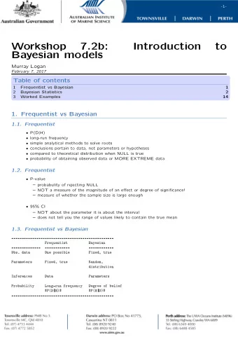
Introduction to Bayesian Statistics Louis Raes Spring 2017 Table - PowerPoint PPT Presentation
Introduction to Bayesian Statistics Louis Raes Spring 2017 Table of contents Organisation, goals What is Bayesian Statistics? Introduction Statistical basics Doing Bayesian Analysis Conjugacy Grid approximation Metropolis algorithm Gibbs
Introduction to Bayesian Statistics Louis Raes Spring 2017
Table of contents Organisation, goals What is Bayesian Statistics? Introduction Statistical basics Doing Bayesian Analysis Conjugacy Grid approximation Metropolis algorithm Gibbs Sampling
Organisation • Small group; very advanced students • Lecture: introduce some concepts, ideas → readings at home and assignments → assignments are not graded • Course is evaluated based on an oral exam; last lecture, exam requirements are handed out → bunch of questions (much overlap with assignments) are handed out → prepare a few for the exam
Teaching Style • Throughout the slides I have put questions (in red). → I expect you to solve these in class (I will pause) → Someone will have to provide the solution to class mates in class → Question too easy? No problem, just solve them, won’t take long → Struggle with a question: indication that you need to read up on this; I refer to chapters and pages from books which may be helpful. A reader with selected readings is provided.
Teaching Style • Questions in blue are not solved in class but need to be done at home. Prepare them for next lecture. I expect students to have solved the blue questions and have answers (or attempts) with them. You are allowed to prepare in groups of two. (In case of abuse, I’ll toughen requirements).
Organisation • Bayesian inference means computation. • Feel free to choose your language / computing environment → R and Matlab are good choices; I use R → your choice is your own responsibility • Tons of resources online; do not mindlessly copy-paste. → In practice I too use a lot from online and offline resources, though the hope is that is not mindlessly done.
Goals • Have an idea about Bayesian inference. • Develop intuition about basic concepts. • After these lectures you should be able to move quicker in case of self-study; if you do not pursue this further at least you have an idea.
Goals • Pace is (relatively) slow, getting fundamentals right. • Do not forget readings, integral part of the course (and exam)
Further resources • Doing Bayesian Data Analysis, John Kruschke Shorthand: Kruschke → Easiest resource on Bayesian Inference I am aware off → Geared towards psychologists → Quirky (humor, poetry) → Super accessible; focus on R → Choice of topics might be a bit erratic, not ideal for economics applications, unless you do experiments (warning: → no idea about usage of Bayes among experimentalists)
Further resources • Bayesian Analysis for the Social Sciences, Simon Jackman Shorthand: Jackman → Graduate level, many applications in political science → Good blend of theory (more formal) and applications → Not too easy; focus on R and Bugs/Jags (Bugs is a bit outdated by now → check out Stan)
Further resources • Bayesian Data Analysis, Gelman et al. Shorthand: BDA → ”The” textbook on Bayesian Statistics; scholar.google: 19318 cites (5/5/2017) → Very comprehensive but with applied bending → Covers applications in many fields • For applications in economics and materials geared towards econometrics → Gary Koop → leading Bayesian, many syllabi, papers, textbooks, codes (Matlab)
Introduction Bayesian inference means using Bayes’s theorem to update beliefs regarding an object of interest after observing data. prior beliefs → data → posterior beliefs ???
Introduction Bayesian inference means practical methods to make inferences from data we observe via probability models, to learn about quantities we are interested in. Three steps: 1. Set up a full probability model: a joint distribution for all observable and nonobservable quantities, consistent with our knowledge about the problem as well as the data collection process 2. Condition on the observed data: the posterior 3. Evaluate model fit and implications of the posterior distribution: does the model fit the data, reasonable conclusions, sensitive? → if necessary, go back to step 1. ( See BDA chapter 1 )
Introduction • Bayesian statistics is often preferred due to philosophical reasons , many disciplines are moving towards interval estimation rather than hypothesis testing and the Bayesian probability interval is much closer to the (common-sense) interpretation of what a confidence interval should be . Question: 1. In a classic (frequentist setting), what is the interpretation of a confidence interval? 2. What is the interpretation of a p -value. Write this down carefully -in your own words.
Introduction Ignoring philosophical discussions, Bayesian inference has other advantages: (i) flexible and general → deal with very complicated problems; (ii) take uncertainty seriously → uncertainty in derived quantities (iii) pooling / shrinkage.
Introduction • To have a meaningful discussion on the merits, we need to introduce quite a bit of jargon. • Philosophical discussions and comparisons with other approaches are to be discussed later onwards.
Introduction Assignment: 1. Read the Introduction of Jackman’s book as well as chapter 1 until p.8
Concepts Question: 1. Write down the definition of conditional probability. 2. Write down an example highlighting / explaining this. 3. What is the law of total probability? 4. What is Bayes’ rule.
Introduction Definition: Let A and B be events with P ( B ) > 0, then the conditional probability of A given B is: P ( A | B ) = P ( A ∩ B ) . (1) P ( B ) While we state it as a definition, it can be justified with a betting argument following de Finetti or derived from more elementary axioms.
Introduction Definition: Multiplication rule P ( A ∩ B ) = P ( A | B ) P ( B ) (2) Definition: Law of total probability P ( B ) = P ( A ∩ B ) + P ( ¬ A ∩ B ) = P ( B | A ) P ( A ) + P ( B |¬ A ) P ( ¬ A ) (3)
Introduction Bayes’s Theorem: If A and B are events with P ( B ) > 0, then P ( A | B ) = P ( B | A ) P ( A ) (4) P ( B ) Proof: . . .
Introduction In Bayesian Statistics we use the above theorem as follows. Let A denote a hypothesis, and B the evidence, then we see that the theorem provides the probability of the hypothesis A after having seen the data B .
Introduction A common illustration is a (drug) testing example. Do this yourself. Write down a reasonable rate for false negatives of a drug test and a reasonable rate of false positives. Choose a true rate of drug use in a subject pool (think of students taking some meds during exam period or athletes). Now derive the posterior probability for a subject, randomly drawn from a subject pool for testing, returning a positive test. What is the probability that the subject has used a substance? Does the result align with your a priori intuition?
Introduction In our research we often work in a continuous setting and we consider continuous parameters we want to learn about: a regression coefficient or proportion etc. Let θ denote the parameter we want to learn about and y = ( y 1 , . . . , y n ) ′ the data at hand. Beliefs are represented as probability density functions or pdf’s. So the prior on θ is p ( θ ) and the posterior is p ( θ | y ). Bayes’s Theorem: p ( y | θ ) p ( θ ) p ( θ | y ) = (5) � p ( y | θ ) p ( θ ) d θ Proof: . . .
Introduction Often this is written as p ( θ | y ) ∝ p ( y | θ ) p ( θ ) , (6) where the constant of proportionality (the denominator missing here), ensures that the posterior integrates to 1, as a proper density must. Furthermore, the term p ( y | θ ) is nothing more than the likelihood. Hence the mantra: the posterior is proportional to the prior times the likelihood .
Introduction A practical example: Coin tossing. What is the chance that a coin comes up heads? → two possibilities that are mutually exclusive → each datum is independent ∼ proportion of babies that are girls ∼ proportion of heart surgery patients who survive after 1 year
Introduction Step 1: specify the likelihood: The probability of a coin coming up heads is a function of an unknown parameter θ : p ( y = 1 | θ ) = f ( θ ) (7) We assume the identify function, so we have p ( y = 1 | θ ) = θ and also p ( y = 0 | θ ) = 1 − θ . Combined we have the Bernoulli distribution: p ( y | θ ) = θ y (1 − θ ) 1 − y
Introduction When we flip a coin N times, we have N observations, so we get: � � θ y i (1 − θ ) 1 − y i p ( { y 1 , . . . , y n }| θ ) = p ( y i | θ ) = (8) i i or write with z the number of times head shows up in N flips, and we get: p ( z , N | θ ) = θ z (1 − θ ) ( N − z ) (9)
Introduction So we have a likelihood, now we need a prior. The key requirement for this prior is that it lives on the interval [0 , 1]. Why?
Introduction So we have a likelihood, now we need a prior. The key requirement for this prior is that it lives on the interval [0 , 1]. Why? → Remember: the posterior can only exist over the support of the prior!
Introduction Proposal: the Beta distrbution: p ( θ | a , b ) = beta( θ | a , b , ) = θ ( a − 1) (1 − θ ) ( b − 1) / B ( a , b ) (10)
Introduction The beta distribution depends on two parameters, B ( a , b ) is a normalizing constant ensures that the area under the density � 1 0 θ ( a − 1) (1 − θ ) ( b − 1) d θ integrates to 1: B ( a , b ) = mean: ¯ θ = a / ( a + b )
Recommend
More recommend
Explore More Topics
Stay informed with curated content and fresh updates.


