Introduction to Artificial Intelligence Unsupervised Learning Janyl - - PowerPoint PPT Presentation

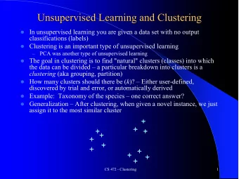
Introduction to Artificial Intelligence Unsupervised Learning

Janyl Jumadinova October 21, 2016

Supervised learning vs. Unsupervised learning

◮ Supervised learning: discover patterns in the data that relate

data attributes with a target (class) attribute.

• These patterns are then utilized to predict the values of the

target attribute in future data instances.

2/29

Supervised learning vs. Unsupervised learning

◮ Supervised learning: discover patterns in the data that relate

data attributes with a target (class) attribute.

• These patterns are then utilized to predict the values of the

target attribute in future data instances.

◮ Unsupervised learning: the data has no target attribute.

• We want to explore the data to find some intrinsic structures

in them.

2/29

Clustering

◮ Organizing data into classes such that there is:

• high intra-class similarity
• low inter-class similarity

3/29

Clustering

◮ Organizing data into classes such that there is:

• high intra-class similarity
• low inter-class similarity

◮ Finding the class labels and the number of classes directly from

the data (in contrast to classification).

3/29

Clustering

◮ Organizing data into classes such that there is:

• high intra-class similarity
• low inter-class similarity

◮ Finding the class labels and the number of classes directly from

the data (in contrast to classification).

◮ More informally, finding natural groupings among objects. 3/29

Clustering

Clustering is one of the most utilized data mining techniques

It has a long history, and used in almost every field, e.g., medicine, psychology, botany, sociology, biology, archeology, marketing, insurance, libraries, etc.

4/29

Clustering

Clustering is one of the most utilized data mining techniques

It has a long history, and used in almost every field, e.g., medicine, psychology, botany, sociology, biology, archeology, marketing, insurance, libraries, etc.

◮ Ex.: : Given a collection of text documents, we want to

• rganize them according to their content similarities.

4/29

Clustering

Clustering is one of the most utilized data mining techniques

It has a long history, and used in almost every field, e.g., medicine, psychology, botany, sociology, biology, archeology, marketing, insurance, libraries, etc.

◮ Ex.: : Given a collection of text documents, we want to

• rganize them according to their content similarities.

◮ Ex.: In marketing, segment customers according to their

similarities (to do targeted marketing).

4/29

What is a natural grouping among these

• bjects?

5/29

What is a natural grouping among these objects?

6/29

What is Similarity?

7/29

What is Similarity?

The quality or state of being similar; likeness; resemblance; as, a similarity

• f features. Webster’s Dictionary

7/29

What is Similarity?

The quality or state of being similar; likeness; resemblance; as, a similarity

• f features. Webster’s Dictionary

7/29

What is Similarity?

The quality or state of being similar; likeness; resemblance; as, a similarity

• f features. Webster’s Dictionary

Similarity is hard to define, but ... “We know it when we see it” The real meaning of similarity is a philosophical question. We will take a more pragmatic approach. 7/29

Defining Distance Measures

Definition:

Let O1 and O2 be two objects from the universe of possible objects. The distance (dissimilarity) between O1 and O2 is a real number denoted by D(O1, O2).

8/29

What properties should a distance measure have?

◮ D(A, B) = D(B, A)

Symmetry

Otherwise you could claim “Greg looks like Oliver, but Oliver looks nothing like Greg.” 9/29

What properties should a distance measure have?

◮ D(A, B) = D(B, A)

Symmetry

Otherwise you could claim “Greg looks like Oliver, but Oliver looks nothing like Greg.” ◮ D(A, A) = 0

Constancy of Self-Similarity

Otherwise you could claim “Greg looks more like Oliver, than Oliver does.” 9/29

What properties should a distance measure have?

◮ D(A, B) = D(B, A)

Symmetry

Otherwise you could claim “Greg looks like Oliver, but Oliver looks nothing like Greg.” ◮ D(A, A) = 0

Constancy of Self-Similarity

Otherwise you could claim “Greg looks more like Oliver, than Oliver does.” ◮ D(A, B) = 0 iff A = B

Positivity (Separation)

Otherwise there are objects in your world that are different, but you cannot tell apart. 9/29

What properties should a distance measure have?

◮ D(A, B) = D(B, A)

Symmetry

Otherwise you could claim “Greg looks like Oliver, but Oliver looks nothing like Greg.” ◮ D(A, A) = 0

Constancy of Self-Similarity

Otherwise you could claim “Greg looks more like Oliver, than Oliver does.” ◮ D(A, B) = 0 iff A = B

Positivity (Separation)

Otherwise there are objects in your world that are different, but you cannot tell apart. ◮ D(A, B) ≤ D(A, C) + D(B, C)

Triangular Inequality

Otherwise you could claim “Greg is very like Bob, and Greg is very like Oliver, but Bob is very unlike Oliver.” 9/29

How do we measure similarity?

10/29

How do we measure similarity?

To measure the similarity between two objects, transform one of the

• bjects into the other, and measure how much effort it took. The

measure of effort becomes the distance measure.

11/29

How do we measure similarity?

12/29

Partitional Clustering

◮ Non-hierarchical, each instance is placed in exactly one of K

nonoverlapping clusters.

◮ Since only one set of clusters is output, the user normally has to

input the desired number of clusters K.

13/29

Minimize Squared Error

14/29

K-means clustering

◮ K-means is a partitional clustering algorithm. ◮ The k-means algorithm partitions the given data into k clusters.

◮ Each cluster has a cluster center, called centroid. ◮ k is specified by the user.

15/29

K-means Algorithm

• 1. Decide on a value for k.

16/29

K-means Algorithm

• 1. Decide on a value for k.
• 2. Initialize the k cluster centers (randomly, if necessary).

16/29

K-means Algorithm

• 1. Decide on a value for k.
• 2. Initialize the k cluster centers (randomly, if necessary).
• 3. Decide the class memberships of the N objects by assigning

them to the nearest cluster center.

16/29

K-means Algorithm

• 1. Decide on a value for k.
• 2. Initialize the k cluster centers (randomly, if necessary).
• 3. Decide the class memberships of the N objects by assigning

them to the nearest cluster center.

• 4. Re-estimate the k cluster centers, by assuming the memberships

found above are correct.

16/29

K-means Algorithm

• 1. Decide on a value for k.
• 2. Initialize the k cluster centers (randomly, if necessary).
• 3. Decide the class memberships of the N objects by assigning

them to the nearest cluster center.

• 4. Re-estimate the k cluster centers, by assuming the memberships

found above are correct.

• 5. If none of the N objects changed membership in the last

iteration, exit. Otherwise goto 3.

16/29

K-Means Clustering: Step 1

17/29

K-Means Clustering: Step 2

18/29

K-Means Clustering: Step 3

19/29

K-Means Clustering: Step 4

20/29

K-Means Clustering: Step 5

21/29

How can we tell the right number of clusters?

◮ In general, this is an unsolved problem. 22/29

How can we tell the right number of clusters?

◮ In general, this is an unsolved problem. 22/29

How can we tell the right number of clusters?

◮ In general, this is an unsolved problem. ◮ We can use approximation methods! 22/29

23/29

24/29

25/29

We can plot the objective function values for k = 1...6

◮ The abrupt change at k = 2, is highly suggestive of two clusters

in the data.

◮ This technique for determining the number of clusters is known

as “knee finding” or “elbow finding”.

26/29

Strengths of K-Means

◮ Simple: easy to understand and to implement ◮ Efficient: Time complexity O(tkn), where n is the number of

data points, k is the number of clusters, and t is the number of iterations.

• Since both k and t are small, k-means is considered a linear

algorithm.

◮ Often terminates at a local optimum.

• The global optimum may be found using techniques such as:

deterministic annealing and genetic algorithms

27/29

Weaknesses of K-Means

◮ The algorithm is only applicable if the mean is defined.

• For categorical data - the centroid is represented by most

frequent values.

• The user needs to specify k.

28/29

Weaknesses of K-Means

◮ The algorithm is only applicable if the mean is defined.

• For categorical data - the centroid is represented by most

frequent values.

• The user needs to specify k.

◮ The algorithm is sensitive to outliers.

• Outliers are data points that are very far away from other data

points.

• Outliers could be errors in the data recording or some special

data points with very different values.

28/29

K-Means Summary

◮ Despite weaknesses, k-means is still the most popular algorithm

due to its simplicity, efficiency and other clustering algorithms have their own lists of weaknesses.

◮ No clear evidence that any other clustering algorithm performs

better in general, although they may be more suitable for some specific types of data or applications.

◮ Comparing different clustering algorithms is a difficult task. No

• ne knows the correct clusters!

29/29