Introduction to Artificial Intelligence Local Search Janyl - PowerPoint PPT Presentation

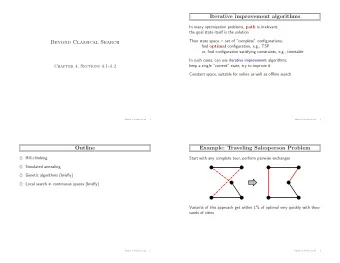
Introduction to Artificial Intelligence Local Search Janyl Jumadinova September 19, 2016

Evaluation ◮ Completeness : Is the algorithm guaranteed to find a solution when there is one? ◮ Optimality : Does the strategy find the optimal solution? ◮ Time complexity : How long does it take to find a solution? ◮ Space complexity : How much memory is needed to perform the search? 2/18

Search Summary Name Complete Optimal Time Space O ( b d ) O ( b d ) BFS Yes* Yes* O ( b m ) DFS No No O ( bm ) O ( b m )* O ( b m ) Greedy best-first No No A* Yes* Yes* exp. exp. b is the branching factor/maximum number of successors of any node, d is the depth of the shallowest solution, m is the maximum depth of the tree * indicates that there is a special case where this may not be true 3/18

Local Search Local search algorithms ◮ operate using a single current node (rather than multiple paths) ◮ generally move only to neighbors of that node 4/18

Local Search Benefits 1. use very little memory (usually a constant amount) 2. can often find reasonable solutions in large or infinite (continuous) state spaces for which systematic algorithms are unsuitable 3. useful for solving pure optimization problems, where the aim is to find the best state according to an objective function 5/18

Local Search objective function global maximum shoulder local maximum "flat" local maximum state space current state 6/18

Hill-Climbing Or gradient ascent/descent Also known as “Like climbing Everest in thick fog with amnesia” objective function global maximum shoulder local maximum "flat" local maximum state space current state 7/18

Hill-Climbing ◮ A loop that continually moves in the direction of increasing value that is, uphill. ◮ It terminates when it reaches a “peak” where no neighbor has a higher value. 8/18

Hill-Climbing ◮ A loop that continually moves in the direction of increasing value that is, uphill. ◮ It terminates when it reaches a “peak” where no neighbor has a higher value. ◮ The algorithm does not maintain a search tree, so the data structure for the current node need only record the state and the value of the objective function. 8/18

Hill-Climbing ◮ A loop that continually moves in the direction of increasing value that is, uphill. ◮ It terminates when it reaches a “peak” where no neighbor has a higher value. ◮ The algorithm does not maintain a search tree, so the data structure for the current node need only record the state and the value of the objective function. ◮ Hill climbing does not look ahead beyond the immediate neighbors of the current state. 8/18

Hill-Climbing 9/18

Implementing Hill-Climbing: Environment Setup Let’s start with a model we built a week ago (on September 12) First we will create a background by re-writing the set-up procedure: patches-own [elevation] to setup ca setup-patches setup-turtles reset-ticks end 10/18

We need to define setup-patches and setup-turtles procedures: to setup-patches ask patches [ set elevation (random 10000) ] diffuse elevation 1 ask patches [ set pcolor scale-color green elevation 1000 9000 ] end to setup-turtles crt 100 ask turtles [ if (shade-of? green color) [ set color red ] setxy random-xcor random-ycor ] end 11/18

We need to define and display the highest and lowest points in our terrain: globals [highest ;; the highest patch elevation lowest] ;; the lowest patch elevation - Let’s set up two monitors in the Interface tab with the Toolbar ( highest and lowest ) 12/18

Modify the setup-patches procedure: to setup-patches ask patches [ set elevation (random 10000) ] diffuse elevation 1 ask patches [ set pcolor scale-color green elevation 1000 9000 ] set highest max [elevation] of patches set lowest min [elevation] of patches ask patches [ if (elevation > (highest - 100)) [set pcolor white] if (elevation < (lowest + 100)) [set pcolor black] ] end 13/18

Hill-climbing 1. The turtles cannot see ahead farther than just one patch 2. Each turtle can move only one square each turn 3. Turtles are blissfully ignorant of each other ;; each turtle goes to the highest elev-n in a radius of 1 to move-to-local-max ask turtles [ uphill elevation if ( [elevation] of patch-ahead 1 > elevation ) [ fd 1 ] ] end 14/18

Hill-climbing ◮ Every patch picked a random elevation, and then we diffused these values one time ◮ This doesn’t provide a continuous spread of elevation across the graphics window ◮ So, we diffuse more! repeat 5 [ diffuse elevation 1 ] 15/18

Hill-climbing Let’s plot the number of turtles who have reached the ’peak-zone’ (within 1% of the highest elevation) to do-plots set-current-plot "Turtles at Peaks" plot count turtles with [ elevation >= (highest - 100) ] end - Create a slider for the number of turtles and replace the hard-coded value with it 16/18

Hill-climbing We may want to stop the model after all the turtles have found their local maxima - Add turtles-moved? variable to global variables - At the end of the go procedure, add a test to see if any turtles have moved to go set turtles-moved? false move-to-local-max do-plots if (not turtles-moved?) [ stop ] end 17/18

Other Search Algorithms Category Name Uninformed Search Uniform-Cost Uninformed Search Depth-limited Uninformed Search Iterative Deepening DFS Uninformed Search Bidirectional Informed Search Iterative-deepening A* Informed Search Recursive best-first search Informed Search Simplified memory-bounded A* Local Search Simulated annealing Local Search Local beam search Local Search Genetic algorithm 18/18