Introduction: Bayesian vs frequentist data analysis Shravan - PowerPoint PPT Presentation

Introduction: Bayesian vs frequentist data analysis Shravan Vasishth Cognitive Science / Linguistics University of Potsdam, Germany www.ling.uni-potsdam.de/~vasishth

A bit about myself 1. Professor of Linguistics at Potsdam 2. Background in Japanese, Computer Science, Statistics 3. Current research interests •Computational models of language processing •Understanding comprehension deficits in aphasia •Applications of Bayesian methods to data analysis •Teaching Bayesian methods to non-experts 2

The main points of this lecture 1. Frequentist methods work well when power is high 2. When power is low, frequentist methods break down 3. Bayesian methods are useful when power is low 4. Why are Bayesian methods to be preferred? • answer the question directly • focus on uncertainty quantification • are more robust and intuitive 5. I illustrate these points with simple examples 3

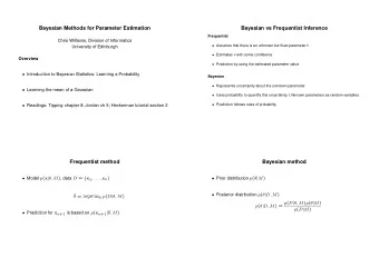
The frequentist procedure Imagine that you have some independent and identically distributed data: x 1 , x 2 , …, x n X ∼ Normal ( μ , σ ) 1. Set up a null hypothesis: H 0 : μ = 0 2. Check if sample mean is consistent with null x ¯ 3. If inconsistent with null, accept specific alternative Statistical data analysis is reduced to checking for significance (is p<0.05?) 4

The frequentist procedure Decision: Reject null and publish X ∼ Normal ( μ , σ ) 5

The frequentist procedure Decision: Reject null and publish X ∼ Normal ( μ , σ ) 6

The frequentist procedure Accept null? Publish or (more likely) put into file drawer X ∼ Normal ( μ , σ ) 7

The frequentist procedure Power: the probability of detecting a particular effect (simplifying a bit) The frequentist paradigm works when power is high (80% or higher). The frequentist paradigm is not designed to be used in low power situations. 8

Low power leads to exaggerated estimates: Type M error (simulated data) Estimates True effect 15 ms, SD 100, 100 (msec) n=20, power=0.10 50 0 − 50 − 100 0 10 20 30 40 50 Sample id Gelman & Carlin, 2014 9

Compare with a high power situation 10

The frequentist paradigm breaks down when power is low 1. Null results are inconclusive 2. Significant results are based on biased estimates (Type M error) Consequences: 1. Non-replicable results 2. Incorrect inferences 11

The frequentist paradigm breaks down when power is low A widely held but incorrect belief: “A significant result (p<0.05) reduces the probability of the null being true” [switch to shiny app by Daniel Schad] https://danielschad.shinyapps.io/probnull/ Under low power, even if we get a significant effect, our belief about the null hypothesis should not change much! 12

Example 1 of a replication of a low-powered study 13 Jäger, Mertzen, Van Dyke & Vasishth, MS, 2018

Example 2 of a replication of a low-powered study 14 Vasishth, Mertzen, Jäger, Gelman, JML 2018

Example 3 of a replication attempt of a low-powered study 15 Vasishth, Mertzen, Jäger, Gelman, JML 2018

The Bayesian approach Imagine again that you have some independent and identically distributed data: x 1 , x 2 , …, x n X ∼ Normal ( μ , σ ) 1. Define prior distributions for the parameters μ , σ 2. Derive posterior distribution of the parameter(s) of interest using Bayes’ rule: f ( μ | data ) ∝ f ( data | μ ) × f ( μ ) posterior likelihood prior 16 3. Carry out inference based on the posterior

Example: Modeling mortality after surgery Modeling prior knowledge: - Suppose we know that 3 out of 30 patients will die after a particular operation - This prior knowledge can be represented as a Beta(3,27) distribution 17

Example: Modeling mortality after surgery Modeling prior knowledge: 18

Example: Modeling mortality after surgery 19

Example: Modeling mortality after surgery The data : 0 deaths in the next 10 operations. The posterior distribution of the probability of death: Posterior ∝ Likelihood × Prior 20

Example: Modeling mortality after surgery Suppose that Prior probability of death was higher: 21

Example: Modeling mortality after surgery The data : 0 deaths in the next 10 operations. The posterior distribution of the probability of death: Posterior ∝ Likelihood × Prior 22

Example: Modeling mortality after surgery The data : 0 deaths in the next 300 operations. The posterior distribution of the probability of death: 23

Summary The posterior is a compromise between the prior and the data When data are sparse, the posterior reflects the prior When a lot of data is available, the posterior reflects the likelihood 24

Hypothesis testing using the Bayes factor We may want to compare two alternative models: Model 1 : Probability of death = 0.5 Model 2 : Probability of death ∼ Beta (1,1) BF 12 = Prob ( Data | Model 1) Bayes factor: Prob ( Data | Model 2) 25

Hypothesis testing using the Bayes factor Model 1 : Probability of death = 0.5 k ) θ 0 (1 − θ ) 10 = ( ( 0 ) 0.5 10 = 0.000977 n 10 Model 2 : Probability of death ∼ Beta (1,1) (Some calculus needed here) 1 11 BF 12 = Prob ( Data | Model 1) Prob ( Data | Model 2) = 0.000977 = 0.01 1/11 Model 2 is 10 times more likely than Model 1 26

Comparison of Frequentist vs Bayesian approaches 27

Some advantages of the Bayesian approach 1. Handles sparse data without any problems 2. Highly customised models can be defined 3. The focus is on uncertainty quantification 4. Answers the research question directly 28

Some disadvantages of the Bayesian approach 1. You have to understand what you are doing •Distribution theory •Random variable theory •Maximum likelihood estimation •Linear modeling theory 2. Requires programming ability •Statistical computing using Stan (mc-stan.org) 3. Computational cost •Cluster computing is sometimes needed •GPU based computing is coming in 2019 4. Priors require thought •Eliciting priors from experts •Adversarial analyses 29