Interactions In the additive model, the effect of one factor is not - PowerPoint PPT Presentation

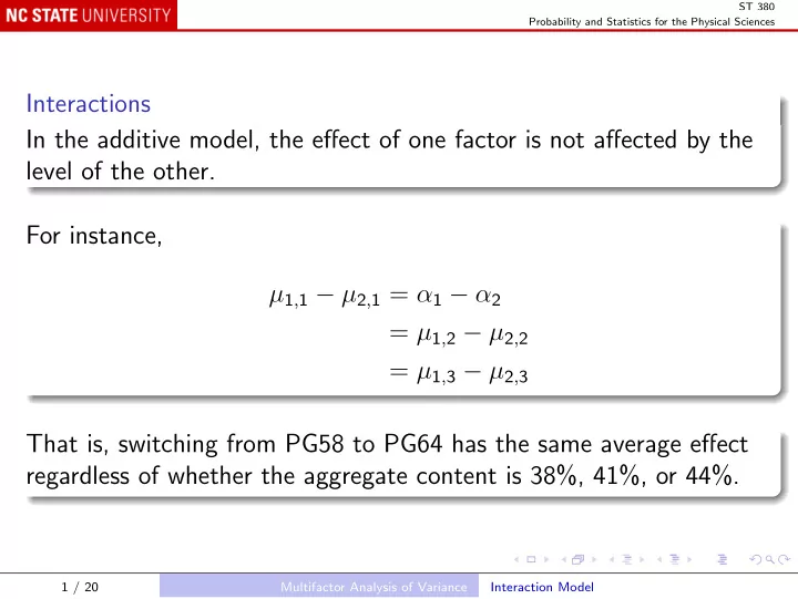
ST 380 Probability and Statistics for the Physical Sciences Interactions In the additive model, the effect of one factor is not affected by the level of the other. For instance, µ 1 , 1 − µ 2 , 1 = α 1 − α 2 = µ 1 , 2 − µ 2 , 2 = µ 1 , 3 − µ 2 , 3 That is, switching from PG58 to PG64 has the same average effect regardless of whether the aggregate content is 38%, 41%, or 44%. 1 / 20 Multifactor Analysis of Variance Interaction Model

ST 380 Probability and Statistics for the Physical Sciences The additive model is not always appropriate: in many problems, the effect of one factor is affected by the level of the other. In this case, we say the the factors interact with each other. Synergy of drugs is an example of interaction: if the effect of two drugs taken together is greater than the sum of their individual effects, they are synergistic . 2 / 20 Multifactor Analysis of Variance Interaction Model

ST 380 Probability and Statistics for the Physical Sciences We can explore possible interactions using an interaction plot of the 9 treatment means: with(asphalt, interaction.plot(AsphGr, AggCont, Cond)) or with(asphalt, interaction.plot(AggCont, AsphGr, Cond)) The effect of binder grade appears to diminish as the coarse aggregate content is increased. If there were no interaction, the graphs would be parallel. 3 / 20 Multifactor Analysis of Variance Interaction Model

ST 380 Probability and Statistics for the Physical Sciences The Interaction Model To test the significance of the interactions, we extend the additive model to the interaction model : µ i , j = E ( X i , j , k ) = µ + α i + β j + γ i , j , k = 1 , 2 , where the additional parameters γ i , j must also be constrained: in R: γ i , 1 = 0 , i = 1 , 2 , . . . , I γ 1 , j = 0 , j = 1 , 2 , . . . , J in SAS: γ i , J = 0 , i = 1 , 2 , . . . , I γ I , j = 0 , j = 1 , 2 , . . . , J . 4 / 20 Multifactor Analysis of Variance Interaction Model

ST 380 Probability and Statistics for the Physical Sciences We now test the null hypothesis γ i , j = 0 , i = 1 , 2 , . . . , I , j = 1 , 2 , . . . , J . asphaltAov2 <- aov(Cond ~ AsphGr + factor(AggCont) + AsphGr:factor(AggCont), asphalt) summary(asphaltAov2) Output Df Sum Sq Mean Sq F value Pr(>F) AsphGr 2 0.002089 0.001045 14.117 0.00168 ** factor(AggCont) 2 0.008297 0.004149 56.063 8.31e-06 *** AsphGr:factor(AggCont) 4 0.000325 0.000081 1.099 0.41356 Residuals 9 0.000666 0.000074 --- Signif. codes: 0 *** 0.001 ** 0.01 * 0.05 . 0.1 1 5 / 20 Multifactor Analysis of Variance Interaction Model

ST 380 Probability and Statistics for the Physical Sciences The output now has an additional line for AsphGr:factor(AggCont) , which represents the interaction terms γ i , j . There are I × J = 9 interactions, but 5 are constrained to be zero, which is why there are only 4 degrees of freedom. The F -value is small and non-significant, so we do not reject the null hypothesis: the additive model is adequate. The apparent interaction in the plots is no greater than we would expect under the additive model, and can be explained as a chance effect. 6 / 20 Multifactor Analysis of Variance Interaction Model

ST 380 Probability and Statistics for the Physical Sciences Unreplicated Design If the two factors have I and J levels, respectively, and each treatment is replicated K times, the degrees of freedom in the ANOVA table for the interaction model are: Source DF Factor A I − 1 Factor B J − 1 Interactions ( I − 1)( J − 1) Error IJ ( K − 1) Total IJK − 1 If K = 1, there are zero degrees of freedom for error, so no F -tests can be carried out. 7 / 20 Multifactor Analysis of Variance Interaction Model

ST 380 Probability and Statistics for the Physical Sciences However, the degrees of freedom in the ANOVA table for the additive model are: Source DF Factor A I − 1 Factor B J − 1 Error IJ ( K − 1) + ( I − 1)( J − 1) Total IJK − 1 So even if K = 1, there is at least one degree of freedom for error, and the main effects of A and B can be tested. 8 / 20 Multifactor Analysis of Variance Interaction Model

ST 380 Probability and Statistics for the Physical Sciences More Factors Often an experiment is carried out to explore the effects of more than two factors. The additive and interaction models may be generalized accordingly. However, interactions among more than two factors are hard to interpret, so we usually try to find an adequate model with less than all possible interactions. 9 / 20 Multifactor Analysis of Variance More Than Two Factors

ST 380 Probability and Statistics for the Physical Sciences Factorial Design Recall that a treatment is a combination of specific levels of all the factors. If all possible treatments are used, the experiment has a complete factorial design. Since there are I × J × K × . . . treatments, a complete factorial experiment may be infeasible. A fractional factorial design involves a subset of the treatments, usually designed to allow estimation of the main effects of each factor, but perhaps no interactions. 10 / 20 Multifactor Analysis of Variance More Than Two Factors

ST 380 Probability and Statistics for the Physical Sciences Two-Level Designs When a project begins, the effects of many factors may be unknown, but in practice only a few are found to be important. The first phase of experiments are designed to find the factors that are active ; these will be explored more carefully in follow-up experiments. To keep the number of treatments small, usually each factor is used at only two levels. 11 / 20 Multifactor Analysis of Variance More Than Two Factors

ST 380 Probability and Statistics for the Physical Sciences In the dye extraction example, in addition to the time and temperature of the solution step, additional factors are: type of solvent; time and temperature of an evaporation step, in which the dissolved dye is recovered as a solid; time and temperature of a dissolution step, in which the dye is dissolved in a buffer, for transfer to a mass spectrometer. With 7 factors, even if each has only two levels, there are 2 7 = 128 treatments; the complete factorial design is infeasible. 12 / 20 Multifactor Analysis of Variance More Than Two Factors

ST 380 Probability and Statistics for the Physical Sciences A design with 8 = 2 7 − 4 runs allows the additive model to be fitted, but with no degrees of freedom for error. A design with 16 = 2 7 − 3 runs allows the additive model to be fitted, with 8 degrees of freedom for error. To fit the model with two-factor interactions, a design with 64 = 2 7 − 1 runs is needed; it provides 36 degrees of freedom for error. 13 / 20 Multifactor Analysis of Variance More Than Two Factors

ST 380 Probability and Statistics for the Physical Sciences Example 11.16 A quarter-replicate of a 2 5 experiment (2 5 − 2 design) Response is the yield of a chemical process. Factors: A : condensation temperature; B : amount of material B; C : solvent volume; D : condensation time; E : amount of material E. 14 / 20 Multifactor Analysis of Variance More Than Two Factors

ST 380 Probability and Statistics for the Physical Sciences To define the 2 5 − 2 = 8 treatments, begin with the complete 2 3 design in A , B , and C : Treatment A B C 1 -1 -1 -1 2 +1 -1 -1 3 -1 +1 -1 4 +1 +1 -1 5 -1 -1 +1 6 +1 -1 +1 7 -1 +1 +1 8 +1 +1 +1 The low level of any factor is coded -1, and the high level +1. 15 / 20 Multifactor Analysis of Variance More Than Two Factors

ST 380 Probability and Statistics for the Physical Sciences Now define the levels of D and E using the generators D = ABC , E = AC : Treatment D = ABC E = AC A B C 1 -1 -1 -1 -1 +1 2 +1 -1 -1 +1 -1 3 -1 +1 -1 +1 +1 4 +1 +1 -1 -1 -1 5 -1 -1 +1 +1 -1 6 +1 -1 +1 -1 +1 7 -1 +1 +1 -1 -1 8 +1 +1 +1 +1 +1 These generators produce the design in Example 11.16; other generators would produce the other three fractions. 16 / 20 Multifactor Analysis of Variance More Than Two Factors

ST 380 Probability and Statistics for the Physical Sciences Finally, add the observed yields: Treatment A B C D E y 1 -1 -1 -1 -1 +1 23.2 2 +1 -1 -1 +1 -1 16.9 3 -1 +1 -1 +1 +1 16.8 4 +1 +1 -1 -1 -1 15.5 5 -1 -1 +1 +1 -1 23.8 6 +1 -1 +1 -1 +1 23.4 7 -1 +1 +1 -1 -1 16.2 8 +1 +1 +1 +1 +1 18.1 The treatments are listed in a different order in Example 11.17. 17 / 20 Multifactor Analysis of Variance More Than Two Factors

ST 380 Probability and Statistics for the Physical Sciences In R # Begin with A, B, anc C: Ex11.16 <- expand.grid(A = c(-1, 1), B = c(-1, 1), C = c(-1, 1)) # Add D = ABC: Ex11.16 <- within(Ex11.16, D <- A * B * C) # Add E = AC: Ex11.16 <- within(Ex11.16, E <- A * C) # Add the yields: Ex11.16 <- within(Ex11.16, y <- c(23.2, 16.9, 16.8, 15.5, 23.8, 23.4, 16.2, 18.1)) summary(aov(y ~ A + B + C + D + E, Ex11.16)) 18 / 20 Multifactor Analysis of Variance More Than Two Factors

ST 380 Probability and Statistics for the Physical Sciences Output Df Sum Sq Mean Sq F value Pr(>F) A 1 4.65 4.65 0.938 0.4349 B 1 53.56 53.56 10.807 0.0814 . C 1 10.35 10.35 2.089 0.2853 D 1 0.91 0.91 0.184 0.7098 E 1 10.35 10.35 2.089 0.2853 Residuals 2 9.91 4.96 --- Signif. codes: 0 *** 0.001 ** 0.01 * 0.05 . 0.1 1 19 / 20 Multifactor Analysis of Variance More Than Two Factors