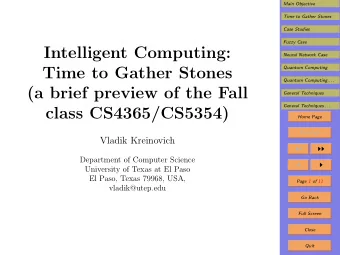
Intelligent Computing: Fuzzy Case Neural Network Case Time to - PowerPoint PPT Presentation
Main Objective Time to Gather Stones Case Studies Intelligent Computing: Fuzzy Case Neural Network Case Time to Gather Stones Quantum Computing (a Tutorial) Proofs (if time allows) Home Page Vladik Kreinovich Title Page
Main Objective 11. Explaining Trapezoid Membership Functions Time to Gather Stones • For each property like “small”: Case Studies Fuzzy Case – first, there are some values which are definitely not Neural Network Case small (e.g., negative ones), Quantum Computing – then some values which are small to some extent; Proofs (if time allows) – then, we have an interval of values which are defi- Home Page nitely small; Title Page – this is followed by values which are somewhat small; ◭◭ ◮◮ – finally, we get values which are absolutely not small. ◭ ◮ • Let us denote the values (“thresholds”) that separate these regions by t 1 , t 2 , t 3 , and t 4 . Page 13 of 147 Go Back • Then: µ ( x ) = 0 for x ≤ t 1 ; µ ( x ) = 1 for t 2 ≤ x ≤ t 3 ; and µ ( x ) = 0 for x ≥ t 4 . Full Screen • Linear interpolation indeed leads to trapezoid func- Close tions. Quit
Main Objective 12. Explaining f & ( a, b ) = a · b Time to Gather Stones Case Studies • If one of the component statements A is false, then the composite statement A & B is also false: f & (0 , b ) = 0. Fuzzy Case Neural Network Case • If A is absolutely true, then our belief in A & B is equiv- Quantum Computing alent to our degree of belief in B : f & (1 , b ) = b . Proofs (if time allows) def • Let us fix b and consider a function F b ( a ) = f & ( a, b ) Home Page that maps a into the value f & ( a, b ). Title Page • We know that F b (0) = 0 and F b (1) = b . ◭◭ ◮◮ • Linear interpolation leads to F b ( a ) = a · b , i.e., to the ◭ ◮ algebraic product f & ( a, b ) = a · b . Page 14 of 147 • Please note that: Go Back – while the resulting operation is commutative and associative, Full Screen – we did not require commutativity or associativity; Close – all we required was linear interpolation. Quit
Main Objective 13. What If We Additionally Require That A & A Time to Gather Stones is Equivalent to A Case Studies • Another intuitive property of “and” is that for every Fuzzy Case B , “ B and B ” means the same as B : f & ( b, b ) = b . Neural Network Case Quantum Computing • We know that F b (0) = f & (0 , b ) = 0 and that F b ( b ) = Proofs (if time allows) f & ( b, b ) = b . Home Page • Thus, on the interval [0 , b ], linear interpolation leads Title Page to F b ( a ) = a , i.e., to f & ( a, b ) = a . ◭◭ ◮◮ • From F b ( b ) = b and F b (1) = f & (1 , b ) = b , we conclude that f & ( a, b ) = F b ( a ) = b for all a ∈ [ b, 1]; so: ◭ ◮ Page 15 of 147 • f & ( a, b ) = a when a ≤ b and • f & ( a, b ) = b when b ≤ a . Go Back Full Screen • Thus, f & ( a, b ) = min( a, b ). Close Quit
Main Objective 14. Linear Interpolation Explains the Usual Choice Time to Gather Stones of t-Conorms Case Studies • If A is absolutely true, then A ∨ B is also absolutely Fuzzy Case true: f ∨ ( a, b ) = f ∨ (1 , b ) = 1. Neural Network Case Quantum Computing • If A is absolutely false, then our belief in A ∨ B is Proofs (if time allows) equivalent to our degree of belief in B : f ∨ (0 , b ) = b . Home Page def • For G b ( a ) = f ∨ ( a, b ), we get G b (0) = b and G b (1) = 1. Title Page • Linear interpolation leads to G b ( a ) = b + a · (1 − b ), ◭◭ ◮◮ i.e., to the algebraic sum f ∨ ( a, b ) = a + b − a · b . ◭ ◮ • Note that: Page 16 of 147 – while the resulting operation is commutative and Go Back associative, Full Screen – we did not require commutativity or associativity, Close – all we required was linear interpolation. Quit
Main Objective 15. What If We Additionally Require That A ∨ A Time to Gather Stones is Equivalent to A Case Studies • Another intuitive property of “or” is that for every B , Fuzzy Case “ B or B ” means the same as B : f ∨ ( b, b ) = b . Neural Network Case Quantum Computing • We know that G b (0) = f ∨ (0 , b ) = b and that G b ( b ) = Proofs (if time allows) f ∨ ( b, b ) = b . Home Page • Thus, for a ∈ [0 , b ], linear interpolation leads to G b ( a ) = Title Page b , i.e., to f & ( a, b ) = b . ◭◭ ◮◮ • From G b ( b ) = b and G b (1) = f ∨ (1 , b ) = 1, we conclude that f & ( a, b ) = G b ( a ) = a for all a ∈ [ b, 1]; so: ◭ ◮ Page 17 of 147 • f ∨ ( a, b ) = b when a ≤ b and • f ∨ ( a, b ) = a when b ≤ a . Go Back Full Screen • Thus, f ∨ ( a, b ) = max( a, b ). Close Quit
Main Objective 16. Simple Linear Interpolation Explains the Usual Time to Gather Stones Choice of Negation Operations Case Studies • For the 2-valued logic, with truth values 1 (“true”) and Fuzzy Case 0 (“false”), the negation operation is easy: Neural Network Case Quantum Computing – the negation of “false” is “true”: f ¬ (0) = 1, and Proofs (if time allows) – the negation of “true” is “false”: f ¬ (1) = 0. Home Page • We want to extend this operation from the 2-valued Title Page set { 0 , 1 } to the whole interval [0 , 1]. ◭◭ ◮◮ • Linear interpolation leads to f ¬ ( a ) = 1 − a. ◭ ◮ • This is exactly the most frequently used negation op- Page 18 of 147 eration in fuzzy logic. Go Back Full Screen Close Quit
Main Objective 17. Simple Linear Interpolation Explains the Usual Time to Gather Stones Choice of Defuzzification Case Studies • The desired control u should be close to reasonable Fuzzy Case control values u : u ≈ u . Neural Network Case Quantum Computing • We have different possible control values u . Proofs (if time allows) • Let us start with a simplified situation in which we Home Page have finitely many equally values u 1 , . . . , u k . Title Page • In this case, we want to find the values u for which ◭◭ ◮◮ u ≈ u 1 , u ≈ u 2 , . . . , u ≈ u k . ◭ ◮ • Since the values u i are different, we cannot get the def exact equality in all k cases: e k = u − u k � = 0. Page 19 of 147 def Go Back • We want the vector e = ( e 1 , . . . , e k ) to be as close to the ideal point (0 , . . . , 0) as possible. Full Screen • The distance between the vector e and the 0 point is Close � e 2 1 + . . . + e 2 equal to k . Quit
Main Objective 18. Defuzzification (cont-d) Time to Gather Stones Case Studies • Minimizing the distance is equivalent to minimizing its k = ( u − u 1 ) 2 + . . . + ( u − u k ) 2 . square e 2 1 + . . . + e 2 Fuzzy Case Neural Network Case • This is the usual Least Squares method. Quantum Computing ( u − u ) 2 du . � • In the continuous case, we get an integral Proofs (if time allows) Home Page • This method works well if all the values u are equally possible. Title Page • In reality, different values u have different degrees of ◭◭ ◮◮ possibility µ ( u ). ◭ ◮ • If u is fully possible ( µ ( u ) = 1), we should keep the Page 20 of 147 term ( u − u ) 2 in the sum. Go Back • If u if completely impossible ( µ ( u ) = 0), we should not Full Screen consider this term at all. Close Quit
Main Objective 19. Defuzzification: Result Time to Gather Stones • In general: Case Studies Fuzzy Case – instead of simply adding the squares, Neural Network Case – we first multiply each square by a weight w ( µ ( u )) Quantum Computing depending on µ ( u ), so that w (1) = 1 and w (0) = 0. Proofs (if time allows) w ( µ ( u )) · ( u − u ) 2 du. � • Thus, we minimize Home Page • Linear interpolation leads to w ( µ ) = µ , so we minimize Title Page � µ ( u ) · ( u − u ) 2 du. ◭◭ ◮◮ ◭ ◮ • Differentiating this expression with respect to u and Page 21 of 147 equating the derivative to 0, we conclude that � Go Back u · µ ( u ) du u = µ ( u ) du . � Full Screen • So, simple linear interpolation explains the usual choice Close of centroid defuzzification. Quit
Main Objective 20. Fuzzy Part: Conclusion Time to Gather Stones • In many real-life situations, we need to process expert Case Studies knowledge. Fuzzy Case Neural Network Case • Experts often describe their knowledge by using impre- Quantum Computing cise (“fuzzy”) terms from natural language. Proofs (if time allows) • For processing such knowledge, Zadeh invented fuzzy Home Page techniques. Title Page • Most efficient practical applications of fuzzy techniques ◭◭ ◮◮ use a specific combination of fuzzy techniques: ◭ ◮ – triangular or trapezoid membership functions, Page 22 of 147 – simple t-norms (min or product), – simple t-conorms (max or algebraic sum), and Go Back – centroid defuzzification. Full Screen • For each of these choices, there exists an explanation Close of why this particular choice is efficient. Quit
Main Objective 21. Conclusion (cont-d) Time to Gather Stones Case Studies • Most efficient applications of fuzzy techniques use: Fuzzy Case – triangular or trapezoid membership functions, Neural Network Case – simple t-norms (min or product), Quantum Computing – simple t-conorms (max or algebraic sum), and Proofs (if time allows) – centroid defuzzification. Home Page • For each of these choices, there exists an explanation Title Page of why this particular choice is efficient. ◭◭ ◮◮ • The usual explanations, however, are different for dif- ◭ ◮ ferent techniques. Page 23 of 147 • We show that all these choices can be explained by the Go Back use of the simplest (linear) interpolation. Full Screen • In our opinion, such a unform explanation makes the Close resulting choices easier to accept (and easier to teach). Quit
Main Objective Part II Time to Gather Stones Neural Network Case Case Studies Fuzzy Case Neural Network Case Quantum Computing Proofs (if time allows) Home Page Title Page ◭◭ ◮◮ ◭ ◮ Page 24 of 147 Go Back Full Screen Close Quit
Main Objective 22. Why Traditional Neural Networks: Time to Gather Stones (Sanitized) History Case Studies • How do we make computers think? Fuzzy Case Neural Network Case • To make machines that fly it is reasonable to look at Quantum Computing the creatures that know how to fly: the birds. Proofs (if time allows) • To make computers think, it is reasonable to analyze Home Page how we humans think. Title Page • On the biological level, our brain processes information ◭◭ ◮◮ via special cells called ]it neurons. ◭ ◮ • Somewhat surprisingly, in the brain, signals are electric Page 25 of 147 – just as in the computer. Go Back • The main difference is that in a neural network, signals are sequence of identical pulses. Full Screen Close Quit
Main Objective 23. Why Traditional NN: (Sanitized) History Time to Gather Stones Case Studies • The intensity of a signal is described by the frequency of pulses. Fuzzy Case Neural Network Case • A neuron has many inputs (up to 10 4 ). Quantum Computing • All the inputs x 1 , . . . , x n are combined, with some loss, Proofs (if time allows) n into a frequency � w i · x i . Home Page i =1 Title Page • Low inputs do not active the neuron at all, high inputs lead to largest activation. ◭◭ ◮◮ • The output signal is a non-linear function ◭ ◮ � n � Page 26 of 147 � y = f w i · x i − w 0 . Go Back i =1 • In biological neurons, f ( x ) = 1 / (1 + exp( − x )) . Full Screen • Traditional neural networks emulate such biological neu- Close rons. Quit
Main Objective 24. Why Traditional Neural Networks: Time to Gather Stones Real History Case Studies • At first, researchers ignored non-linearity and only used Fuzzy Case linear neurons. Neural Network Case Quantum Computing • They got good results and made many promises. Proofs (if time allows) • The euphoria ended in the 1960s when MIT’s Marvin Home Page Minsky and Seymour Papert published a book. Title Page • Their main result was that a composition of linear func- ◭◭ ◮◮ tions is linear (I am not kidding). ◭ ◮ • This ended the hopes of original schemes. Page 27 of 147 • For some time, neural networks became a bad word. Go Back • Then, smart researchers came us with a genius idea: Full Screen let’s make neurons non-linear. Close • This revived the field. Quit
Main Objective 25. Traditional Neural Networks: Main Motiva- Time to Gather Stones tion Case Studies • One of the main motivations for neural networks was Fuzzy Case that computers were slow. Neural Network Case Quantum Computing • Although human neurons are much slower than CPU, Proofs (if time allows) the human processing was often faster. Home Page • So, the main motivation was to make data processing Title Page faster. ◭◭ ◮◮ • The idea was that: ◭ ◮ – since we are the result of billion years of ever im- Page 28 of 147 proving evolution, – our biological mechanics should be optimal (or close Go Back to optimal). Full Screen Close Quit
Main Objective 26. How the Need for Fast Computation Leads to Time to Gather Stones Traditional Neural Networks Case Studies • To make processing faster, we need to have many fast Fuzzy Case processing units working in parallel. Neural Network Case Quantum Computing • The fewer layers, the smaller overall processing time. Proofs (if time allows) • In nature, there are many fast linear processes – e.g., Home Page combining electric signals. Title Page • As a result, linear processing (L) is faster than non- ◭◭ ◮◮ linear one. ◭ ◮ • For non-linear processing, the more inputs, the longer it takes. Page 29 of 147 Go Back • So, the fastest non-linear processing (NL) units process just one input. Full Screen • It turns out that two layers are not enough to approx- Close imate any function. Quit
Main Objective 27. Why One or Two Layers Are Not Enough Time to Gather Stones • With 1 linear (L) layer, we only get linear functions. Case Studies Fuzzy Case • With one nonlinear (NL) layer, we only get functions Neural Network Case of one variable. � n Quantum Computing � • With L → NL layers, we get g � w i · x i − w 0 . Proofs (if time allows) i =1 Home Page • For these functions, the level sets f ( x 1 , . . . , x n ) = const n Title Page � are planes w i · x i = c . ◭◭ ◮◮ i =1 • Thus, they cannot approximate, e.g., f ( x 1 , x 2 ) = x 1 · x 2 ◭ ◮ for which the level set is a hyperbola. Page 30 of 147 n • For NL → L layers, we get f ( x 1 , . . . , x n ) = � f i ( x i ). Go Back i =1 Full Screen ∂ 2 f def • For all these functions, d = = 0, so we also Close ∂x 1 ∂x 2 cannot approximate f ( x 1 , x 2 ) = x 1 · x 2 with d = 1 � = 0. Quit
Main Objective 28. Why Three Layers Are Sufficient: Time to Gather Stones Newton’s Prism and Fourier Transform Case Studies • In principle, we can have two 3-layer configurations: Fuzzy Case L → NL → L and NL → L → NL. Neural Network Case Quantum Computing • Since L is faster than NL, the fastest is L → NL → L: � n Proofs (if time allows) K � � � y = W k · f k w ki · x i − w k 0 − W 0 . Home Page k =1 i =1 Title Page • Newton showed that a prism decomposes while light ◭◭ ◮◮ (or any light) into elementary colors. ◭ ◮ • In precise terms, elementary colors are sinusoids Page 31 of 147 A · sin( w · t ) + B · cos( w · t ) . Go Back • Thus, every function can be approximated, with any Full Screen accuracy, as a linear combination of sinusoids: � Close f ( x 1 ) ≈ ( A k · sin( w k · x 1 ) + B k · cos( w k · x 1 )) . k Quit
Main Objective 29. Why Three Layers Are Sufficient (cont-d) Time to Gather Stones Case Studies • Newton’s prism result: Fuzzy Case � f ( x 1 ) ≈ ( A k · sin( w k · x 1 ) + B k · cos( w k · x 1 )) . Neural Network Case k Quantum Computing • This result was theoretically proven later by Fourier. Proofs (if time allows) • For f ( x 1 , x 2 ), we get a similar expression for each x 2 , Home Page with A k ( x 2 ) and B k ( x 2 ). Title Page • We can similarly represent A k ( x 2 ) and B k ( x 2 ), thus ◭◭ ◮◮ getting products of sines, and it is known that, e.g.: ◭ ◮ cos( a ) · cos( b ) = 1 2 · (cos( a + b ) + cos( a − b )) . Page 32 of 147 • Thus, we get an approximation of the desired form with Go Back f k = sin or f k = cos: Full Screen � n K � � � y = W k · f k w ki · x i − w k 0 . Close k =1 i =1 Quit
Main Objective 30. Which Activation Functions f k ( z ) Should We Time to Gather Stones Choose Case Studies • A general 3-layer NN has the form: Fuzzy Case � n Neural Network Case K � � � y = W k · f k w ki · x i − w k 0 − W 0 . Quantum Computing i =1 k =1 Proofs (if time allows) • Biological neurons use f ( z ) = 1 / (1 + exp( − z )), but Home Page shall we simulate it? Title Page • Simulations are not always efficient. ◭◭ ◮◮ • E.g., airplanes have wings like birds but they do not ◭ ◮ flap them. Page 33 of 147 • Let us analyze this problem theoretically. Go Back • There is always some noise c in the communication Full Screen channel. Close • So, we can consider either the original signals x i or denoised ones x i − c . Quit
Main Objective 31. Which f k ( z ) Should We Choose (cont-d) Time to Gather Stones Case Studies • The results should not change if we perform a full or partial denoising z → z ′ = z − c . Fuzzy Case Neural Network Case • Denoising means replacing y = f ( z ) with y ′ = f ( z − c ). Quantum Computing • So, f ( z ) should not change under shift z → z − c . Proofs (if time allows) Home Page • Of course, f ( z ) cannot remain the same: if f ( z ) = f ( z − c ) for all c , then f ( z ) = const . Title Page • The idea is that once we re-scale x , we should get the ◭◭ ◮◮ same formula after we apply a natural y -re-scaling T c : ◭ ◮ f ( x − c ) = T c ( f ( x )) . Page 34 of 147 Go Back • Linear re-scalings are natural: they corresponding to changing units and starting points (like C to F). Full Screen Close Quit
Main Objective 32. Which Transformations Are Natural? Time to Gather Stones • An inverse T − 1 to a natural re-scaling T c should also Case Studies c be natural. Fuzzy Case Neural Network Case • A composition y → T c ( T c ′ ( y )) of two natural re-scalings Quantum Computing T c and T c ′ should also be natural. Proofs (if time allows) • In mathematical terms, natural re-scalings form a group . Home Page • For practical purposes, we should only consider re- Title Page scaling determined by finitely many parameters. ◭◭ ◮◮ • So, we look for a finite-parametric group containing all ◭ ◮ linear transformations. Page 35 of 147 Go Back Full Screen Close Quit
Main Objective 33. A Somewhat Unexpected Approach Time to Gather Stones • N. Wiener, in Cybernetics , notices that when we ap- Case Studies proach an object, we have distinct phases: Fuzzy Case Neural Network Case – first, we see a blob (the image is invariant under all Quantum Computing transformations); Proofs (if time allows) – then, we start distinguishing angles from smooth Home Page but not sizes (projective transformations); Title Page – after that, we detect parallel lines (affine transfor- mations); ◭◭ ◮◮ – then, we detect relative sizes (similarities); ◭ ◮ – finally, we see the exact shapes and sizes. Page 36 of 147 • Are there other transformation groups? Go Back • Wiener argued: if there are other groups, after billions Full Screen years of evolutions, we would use them. Close • So he conjectured that there are no other groups. Quit
Main Objective 34. Wiener Was Right Time to Gather Stones • Wiener’s conjecture was indeed proven in the 1960s. Case Studies Fuzzy Case • In 1-D case, this means that all our transformations Neural Network Case are fractionally linear: Quantum Computing f ( z − c ) = A ( c ) · f ( z ) + B ( c ) C ( c ) · f ( z ) + D ( c ) . Proofs (if time allows) Home Page • For c = 0, we get A (0) = D (0) = 1, B (0) = C (0) = 0. Title Page • Differentiating the above equation by c and taking c = ◭◭ ◮◮ 0, we get a differential equation for f ( z ): ◭ ◮ − d f dz = ( A ′ (0) · f ( z )+ B ′ (0)) − f ( z ) · ( C ′ (0) · f ( z )+ D ′ (0)) . Page 37 of 147 Go Back d f • So, C ′ (0) · f 2 + ( A ′ (0) − C ′ (0)) · f + B ′ (0) = − dz. Full Screen • Integrating, we indeed get f ( z ) = 1 / (1 + exp( − z )) Close (after an appropriate linear re-scaling of z and f ( z )). Quit
Main Objective 35. How to Train Traditional Neural Networks: Time to Gather Stones Main Idea Case Studies • Reminder: a 3-layer neural network has the form: Fuzzy Case � n Neural Network Case K � � � y = W k · f w ki · x i − w k 0 − W 0 . Quantum Computing i =1 k =1 Proofs (if time allows) • We need to find the weights that best described obser- Home Page � n , y ( p ) � x ( p ) 1 , . . . , x ( p ) vations , 1 ≤ p ≤ P. Title Page • We find the weights that minimize the mean square ◭◭ ◮◮ P � 2 � y ( p ) − y ( p ) def � approximation error E = , where ◭ ◮ NN p =1 � n Page 38 of 147 K � y ( p ) = � � w ki · x ( p ) W k · f − w k 0 − W 0 . Go Back i k =1 i =1 Full Screen • The simplest minimization algorithm is gradient de- Close scent: w i → w i − λ · ∂E . ∂w i Quit
Main Objective 36. Towards Faster Differentiation Time to Gather Stones • To achieve high accuracy, we need many neurons. Case Studies Fuzzy Case • Thus, we need to find many weights. Neural Network Case • To apply gradient descent, we need to compute all par- Quantum Computing tial derivatives ∂E . Proofs (if time allows) ∂w i Home Page • Differentiating a function f is easy: Title Page – the expression f is a sequence of elementary steps, ◭◭ ◮◮ – so we take into account that ( f ± g ) ′ = f ′ ± g ′ , ( f · g ) ′ = f ′ · g + f · g ′ , ( f ( g )) ′ = f ′ ( g ) · g ′ , etc. ◭ ◮ Page 39 of 147 • For a function that takes T steps to compute, comput- ing f ′ thus takes c 0 · T steps, with c 0 ≤ 3. Go Back • However, for a function of n variables, we need to com- Full Screen pute n derivatives. Close • This would take time n · c 0 · T ≫ T : this is too long. Quit
Main Objective 37. Faster Differentiation: Backpropagation Time to Gather Stones • Idea: Case Studies Fuzzy Case – instead of starting from the variables, Neural Network Case – start from the last step, and compute ∂E ∂v for all Quantum Computing intermediate results v . Proofs (if time allows) • For example, if the very last step is E = a · b , then Home Page ∂E ∂a = b and ∂E ∂b = a . Title Page ◭◭ ◮◮ • At each step y , if we know ∂E ∂v and v = a · b , then ◭ ◮ ∂E ∂a = ∂E ∂v · b and ∂E ∂b = ∂E ∂v · a . Page 40 of 147 • At the end, we get all n derivatives ∂E Go Back in time ∂w i Full Screen c 0 · T ≪ c 0 · T · n. Close • This is known as backpropagation . Quit
Main Objective 38. Beyond Traditional NN Time to Gather Stones • Nowadays, computer speed is no longer a big problem. Case Studies Fuzzy Case • What is a problem is accuracy: even after thousands Neural Network Case of iterations, the NNs do not learn well. Quantum Computing • So, instead of computation speed, we would like to Proofs (if time allows) maximize learning accuracy. Home Page • We can still consider L and NL elements. Title Page • For the same number of variables w i , we want to get ◭◭ ◮◮ more accurate approximations. ◭ ◮ • For given number of variables, and given accuracy, we Page 41 of 147 get N possible combinations. Go Back • If all combinations correspond to different functions, we can implement N functions. Full Screen • However, if some combinations lead to the same func- Close tion, we implement fewer different functions. Quit
Main Objective 39. From Traditional NN to Deep Learning Time to Gather Stones • For a traditional NN with K neurons, each of K ! per- Case Studies mutations of neurons retains the resulting function. Fuzzy Case Neural Network Case • Thus, instead of N functions, we only implement Quantum Computing N Proofs (if time allows) K ! ≪ N functions . Home Page • Thus, to increase accuracy, we need to minimize the Title Page number K of neurons in each layer. ◭◭ ◮◮ • To get a good accuracy, we need many parameters, ◭ ◮ thus many neurons. Page 42 of 147 • Since each layer is small, we thus need many layers. Go Back • This is the main idea behind deep learning . Full Screen Close Quit
Main Objective 40. Empirical Formulas Behind Deep Learning Suc- Time to Gather Stones cesses and How They Can Be Justified Case Studies • The general idea of deep learning is natural. Fuzzy Case Neural Network Case • However, any specific formulas that lead to deep learn- Quantum Computing ing successes are purely empirical. Proofs (if time allows) • These formulas need to be explained. Home Page • In this part of the tutorial: Title Page – we list such formulas, and ◭◭ ◮◮ – we briefly mention how the corresponding formulas ◭ ◮ can be explained. Page 43 of 147 Go Back Full Screen Close Quit
Main Objective 41. Rectified Linear Neurons Time to Gather Stones • Traditional neural networks use complex nonlinear neu- Case Studies rons. Fuzzy Case Neural Network Case • On contrast, deep networks utilize rectified linear neu- Quantum Computing rons with the activation function Proofs (if time allows) s 0 ( z ) = max(0 , z ) . Home Page Title Page • Our explanation is that: ◭◭ ◮◮ – this activation function is invariant under re-scaling (changing of the measuring unit) z → λ · x ; ◭ ◮ – moreover, it is, in effect, the only activation func- Page 44 of 147 tion which is this invariant, and Go Back – it is the only activation f-n optimal with respect to Full Screen any scale-invariant optimality criterion. Close Quit
Main Objective 42. Combining Several Results Time to Gather Stones • To speed up the training, the current deep learning Case Studies algorithms use dropout techniques: Fuzzy Case Neural Network Case – they train several sub-networks on different por- Quantum Computing tions of data, and then Proofs (if time allows) – “average” the results. Home Page • A natural idea is to use arithmetic mean for this “av- Title Page eraging”. ◭◭ ◮◮ • However, empirically, geometric mean works much bet- ◭ ◮ ter. Page 45 of 147 • How to explain this empirical efficiency? Go Back • It turns out that Full Screen – this choice is scale-invariant – and, Close – in effect, it is the only scale-invariant choice. Quit
Main Objective 43. Softmax Time to Gather Stones • In deep learning: Case Studies Fuzzy Case – instead of selecting an alternative for which the ob- Neural Network Case jective function f ( x ) is the largest possible, Quantum Computing – we use so-called softmax – i.e., select each alterna- Proofs (if time allows) tive x with probability proportional to exp( α · f ( x )). Home Page • In general, we could select any increasing function F ( z ) Title Page and select probabilities proportional to F ( f ( x )). ◭◭ ◮◮ • So why exponential function is the most successful? ◭ ◮ Page 46 of 147 Go Back Full Screen Close Quit
Main Objective 44. Softmax: Explanation Time to Gather Stones • When we use softmax, the probabilities do not change Case Studies if we simply shift all the values f ( x ). Fuzzy Case Neural Network Case • I.e., if we change them to f ( x ) + c for some c . Quantum Computing • This shift does not change the original optimization Proofs (if time allows) problem. Home Page • Moreover, exponential functions are the only ones which Title Page lead to such shift-invariant selection. ◭◭ ◮◮ • The exponential functions are only ones which optimal ◭ ◮ under a shift-invariant optimality criterion. Page 47 of 147 Go Back Full Screen Close Quit
Main Objective 45. Need for Convolutional Neural Networks Time to Gather Stones • In many practical situations, the available data comes: Case Studies Fuzzy Case – in terms of time series – when we have values mea- Neural Network Case sured at equally spaced time moments – or Quantum Computing – in terms of an image – when we have data corre- Proofs (if time allows) sponding to a grid of spatial locations. Home Page • Neural networks for processing such data are known as Title Page convolutional neural networks . ◭◭ ◮◮ ◭ ◮ Page 48 of 147 Go Back Full Screen Close Quit
Main Objective 46. Need for Pooling Time to Gather Stones • We want to decrease the distortions caused by mea- Case Studies surement errors. Fuzzy Case Neural Network Case • For that, we take into account that usually, the actual Quantum Computing values at nearby points in time or space are close to Proofs (if time allows) each other. Home Page • As a result, Title Page – instead of using the measurement-distorted value ◭◭ ◮◮ at each point, ◭ ◮ – we can take into account that values at nearby points are close, and Page 49 of 147 – combine (“pool together”) these values into a single Go Back more accurate estimate. Full Screen Close Quit
Main Objective 47. Which Pooling Techniques Work Better: Em- Time to Gather Stones pirical Results Case Studies • In principle, we can have many different pooling algo- Fuzzy Case rithms. Neural Network Case Quantum Computing • It turns out that empirically, in general, the most effi- Proofs (if time allows) cient pooling algorithm is max-pooling : Home Page a = max( a 1 , . . . , a m ) . Title Page • The next efficient is average pooling , when we take the ◭◭ ◮◮ arithmetic average a = a 1 + . . . + a m . ◭ ◮ m • In this tutorial, we provide a theoretical explanation Page 50 of 147 for this empirical observation. Go Back • Namely, we prove that max and average poolings are Full Screen indeed optimal. Close Quit
Main Objective 48. Pooling: Towards a Precise Definition Time to Gather Stones • Based on m values a 1 , . . . , a m , we want to generate a Case Studies single value a . Fuzzy Case Neural Network Case • In the case of arithmetic average, we select a for which Quantum Computing a 1 + . . . + a m = a + . . . + a ( m times). Proofs (if time allows) • In general, pooling means that: Home Page – we select some combination operation ∗ and Title Page – we then select the value a for which a 1 ∗ . . . ∗ a m = ◭◭ ◮◮ a ∗ . . . ∗ a ( m times). ◭ ◮ • For example: Page 51 of 147 – if, as a combination operation, we select max( a, b ), Go Back – then the corresponding condition max( a 1 , . . . , a n ) = max( a, . . . , a ) = a describes the max-pooling. Full Screen • From this viewpoint, selecting pooling means selecting Close an appropriate combination operation. Quit
Main Objective 49. Natural Properties of a Combination Opera- Time to Gather Stones tion Case Studies • The combination operation transforms: Fuzzy Case Neural Network Case – two non-negative values – such as intensity of an Quantum Computing image at a given location Proofs (if time allows) – into a single non-negative value. Home Page • The result of applying this operation should not de- Title Page pend on the order in which we combine the values. ◭◭ ◮◮ • Thus, we should have a ∗ b = b ∗ a (commutativity) and ◭ ◮ a ∗ ( b ∗ c ) = ( a ∗ b ) ∗ c (associativity). Page 52 of 147 Go Back Full Screen Close Quit
Main Objective 50. What Does It Mean to Have an Optimal Pool- Time to Gather Stones ing? Case Studies • Optimality means that on the set of all possible com- Fuzzy Case bination operations, we have a preference relation � . Neural Network Case Quantum Computing • A � B means that the operation B is better than (or Proofs (if time allows) of the same quality as) the operation A . Home Page • This relation should be transitive: Title Page – if C is better than B and B is better than A , ◭◭ ◮◮ – then C should be better than A . ◭ ◮ • An operation A is optimal if it is better than (or of the Page 53 of 147 same quality as) any other operation B : B � A . Go Back • For some preference relations, we may have several dif- ferent optimal combination operations. Full Screen • We can then use this non-uniqueness to optimize some- Close thing else. Quit
Main Objective 51. What Is Optimal Pooling (cont-d) Time to Gather Stones Case Studies • Example: Fuzzy Case – if there are several different combination operations Neural Network Case with the best average-case accuracy, Quantum Computing – we can select, among them, the one for which the Proofs (if time allows) average computation time is the smallest possible. Home Page • If after this, we still get several optimal operations, Title Page – we can use the remaining non-uniqueness ◭◭ ◮◮ – to optimize yet another criterion. ◭ ◮ • We do this until we get a final criterion, for which there Page 54 of 147 is only one optimal combination operation. Go Back Full Screen Close Quit
Main Objective 52. Scale-Invariance Time to Gather Stones • Numerical values of a physical quantity depend on the Case Studies choice of a measuring unit. Fuzzy Case Neural Network Case • For example, if we replace meters with centimeters, the Quantum Computing numerical quantity is multiplied by 100. Proofs (if time allows) • In general: Home Page – if we replace the original unit with a unit which is Title Page λ times smaller, ◭◭ ◮◮ – then all numerical values get multiplied by λ . ◭ ◮ • It is reasonable to require that the preference relation Page 55 of 147 should not change if we change the measuring unit. Go Back • Let us describe this requirement in precise terms. Full Screen Close Quit
Main Objective 53. Scale-Invariance (cont-d) Time to Gather Stones Case Studies • If, in the original units, we had the operation a ∗ b , then, in the new units, the operation will be as follows: Fuzzy Case Neural Network Case – first, we transform the value a and b into the new units, so we get a ′ = λ · a and b ′ = λ · b ; Quantum Computing Proofs (if time allows) – then, we combine the new numerical values, getting Home Page ( λ · a ) ∗ ( λ · b ); Title Page – finally, we re-scale the result to the original units, = λ − 1 · (( λ · a ) ∗ ( λ · b )) . def ◭◭ ◮◮ getting aR λ ( ∗ ) b ◭ ◮ • It therefore makes sense to require that if ∗ � ∗ ′ , then for every λ > 0, we get R λ ( ∗ ) � R λ ( ∗ ′ ). Page 56 of 147 Go Back Full Screen Close Quit
Main Objective 54. Shift-Invariance Time to Gather Stones • The numerical values also change if we change the Case Studies starting point for measurements. Fuzzy Case Neural Network Case • For example, when measuring intensity: Quantum Computing – we can measure the actual intensity of an image, Proofs (if time allows) – or we can take into account that there is always Home Page some noise a 0 > 0, and Title Page – use the noise-only level a 0 as the new starting point. ◭◭ ◮◮ • In this case, instead of each original value a , we get a ◭ ◮ new numerical value a ′ = a − a 0 . Page 57 of 147 Go Back Full Screen Close Quit
Main Objective 55. Shift-Invariance (cont-d) Time to Gather Stones Case Studies • If we apply the combination operation in the new units, then in the old units, we get a slightly different result: Fuzzy Case Neural Network Case – first, we transform the value a and b into the new units, so we get a ′ = a − a 0 and b ′ = b − a 0 ; Quantum Computing Proofs (if time allows) – then, we combine the new numerical values, getting Home Page ( a − a 0 ) ∗ ( b − a 0 ); Title Page – finally, we re-scale the result to the original units, ◭◭ ◮◮ def getting aS a 0 ( ∗ ) b = ( a − a 0 ) ∗ ( b − a 0 ) + a 0 . ◭ ◮ • It makes sense to require that the preference relation Page 58 of 147 not change if we simply change the starting point. Go Back • So if ∗ � ∗ ′ , then for every a 0 , we get S a 0 ( ∗ ) � S a 0 ( ∗ ′ ). Full Screen Close Quit
Main Objective 56. Weak Version of Shift-Invariance Time to Gather Stones • Alternatively, we can have a weaker version of this Case Studies “shift-invariance”. Fuzzy Case Neural Network Case • Namely, we require that shifts in a and b imply a pos- Quantum Computing sibly different shift in a ∗ b , i.e., Proofs (if time allows) – if we shift both a and b by a 0 , Home Page – then the value a ∗ b is shifted by some value f ( a 0 ) Title Page which is, in general, different from a 0 . ◭◭ ◮◮ • Now, we are ready to formulation our results. ◭ ◮ Page 59 of 147 Go Back Full Screen Close Quit
Main Objective 57. Definitions Time to Gather Stones • By a combination operation , we mean a commutative, Case Studies associative operation a ∗ b that: Fuzzy Case Neural Network Case – transforms two non-negative real numbers a and b Quantum Computing – into a non-negative real number a ∗ b . Proofs (if time allows) • By an optimality criterion , we need a transitive reflex- Home Page ive relation � on the set of all combination operations. Title Page • We say that a combination operation ∗ opt is optimal ◭◭ ◮◮ w.r.t. � if ∗ � ∗ opt for all combination operations ∗ . ◭ ◮ • We say that � is final if there exists exactly one � - Page 60 of 147 optimal combination operation. Go Back • We say that an optimality criterion is scale-invariant if for all λ > 0 , ∗ � ∗ ′ implies R λ ( ∗ ) � R λ ( ∗ ′ ) , where: Full Screen Close = λ − 1 · (( λ · a ) ∗ ( λ · b )) . def aR λ ( ∗ ) b Quit
Main Objective 58. Definitions and First Result Time to Gather Stones • We say that an optimality criterion is shift-invariant if Case Studies for all a 0 , ∗ � ∗ ′ implies S a 0 ( ∗ ) � S a 0 ( ∗ ′ ) , where: Fuzzy Case Neural Network Case def aS a 0 ( ∗ ) b = (( a − a 0 ) ∗ ( b − a 0 )) + a 0 . Quantum Computing • We say that � is weakly shift-invariant if for every a 0 , Proofs (if time allows) there exists f ( a 0 ) s.t. ∗ � ∗ ′ implies W a 0 ( ∗ ) � W a 0 ( ∗ ′ ) , Home Page def Title Page where aW a 0 ( ∗ ) b = (( a − a 0 ) ∗ ( b − a 0 )) + f ( a 0 ) . ◭◭ ◮◮ • Proposition 1. For every final, scale- and shift-invariant � , the optimal combination operation ∗ is ◭ ◮ a ∗ b = min( a, b ) or a ∗ b = max( a, b ) . Page 61 of 147 Go Back • This result explains why max-pooling is empirically the best combination operation . Full Screen • Note that this result does not contradict uniqueness as Close we requested. Quit
Main Objective 59. Results (cont-d) Time to Gather Stones Case Studies • Indeed, there are several different final scale- and shift- invariant optimality criteria. Fuzzy Case Neural Network Case • For each of these criteria, there is only one optimal Quantum Computing combination operation. Proofs (if time allows) • For some of these optimality criteria, the optimal com- Home Page bination operation is min( a, b ). Title Page • For other criteria, the optimal combination operation ◭◭ ◮◮ is max( a, b ). ◭ ◮ • Proposition 2. For every final, scale-invariant and weakly shift-invariant � , the optimal ∗ is: Page 62 of 147 Go Back a ∗ b = 0 , a ∗ b = min( a, b ) , a ∗ b = max( a, b ) , or Full Screen a ∗ b = a + b. Close • This result explains why max-pooling and average-pooling are empirically the best combination operations . Quit
Main Objective Part III Time to Gather Stones Quantum Computing Case Studies Fuzzy Case Neural Network Case Quantum Computing Proofs (if time allows) Home Page Title Page ◭◭ ◮◮ ◭ ◮ Page 63 of 147 Go Back Full Screen Close Quit
Main Objective 60. Why Quantum Computing Time to Gather Stones • In many practical problems, we need to process large Case Studies amounts of data in a limited time. Fuzzy Case Neural Network Case • To be able to do it, we need computations to be as fast Quantum Computing as possible. Proofs (if time allows) • Computations are already fast. Home Page • However, there are many important problems for which Title Page we still cannot get the results on time. ◭◭ ◮◮ • For example, we can predict with a reasonable accuracy ◭ ◮ where the tornado will go in the next 15 minutes. Page 64 of 147 • However, these computations take days on the fastest Go Back existing high performance computer. Full Screen • One of the main limitations: the speed of all the pro- cesses is limited by the speed of light c ≈ 3 · 10 5 km/sec. Close Quit
Main Objective 61. Why Quantum Computing (cont-d) Time to Gather Stones Case Studies • For a laptop of size ≈ 30 cm, the fastest we can send a 30 cm 3 · 10 5 km / sec ≈ 10 − 9 sec. Fuzzy Case signal across the laptop is Neural Network Case • During this time, a usual few-Gigaflop laptop performs Quantum Computing quite a few operations. Proofs (if time allows) Home Page • To further speed up computations, we thus need to further decrease the size of the processors. Title Page ◭◭ ◮◮ • We need to fit Gigabytes of data – i.e., billions of cells – within a small area. ◭ ◮ • So, we need to attain a very small cell size. Page 65 of 147 • At present, a typical cell consists of several dozen molecules. Go Back • As we decrease the size further, we get to a few-molecule Full Screen size. Close Quit
Main Objective 62. Why Quantum Computing (cont-d) Time to Gather Stones Case Studies • At this size, physics is different: quantum effects be- come dominant. Fuzzy Case Neural Network Case • At first, quantum effects were mainly viewed as a nui- Quantum Computing sance. Proofs (if time allows) • For example, one of the features of quantum world is Home Page that its results are usually probabilistic. Title Page • So, if we simply decrease the cell size but use the same ◭◭ ◮◮ computer engineering techniques, then: ◭ ◮ – instead of getting the desired results all the time, Page 66 of 147 – we will start getting other results with some prob- Go Back ability. Full Screen • This probability of undesired results increases as we decrease the size of the computing cells. Close Quit
Main Objective 63. Why Quantum Computing (cont-d) Time to Gather Stones Case Studies • However, researchers found out that: Fuzzy Case – by appropriately modifying the corresponding al- Neural Network Case gorithms, Quantum Computing – we can avoid the probability-related problem and, Proofs (if time allows) even better, make computations faster. Home Page • The resulting algorithms are known as algorithms of Title Page quantum computing . ◭◭ ◮◮ ◭ ◮ Page 67 of 147 Go Back Full Screen Close Quit
Main Objective 64. Lemon into Lemonade Time to Gather Stones • In non-quantum computing, finding an element in an Case Studies unsorted database with n entries may require time n . Fuzzy Case Neural Network Case • Indeed, we may need to look at each record. Quantum Computing • In quantum computing, it is possible to find this ele- Proofs (if time allows) ment in much smaller time √ n . Home Page Title Page ◭◭ ◮◮ ◭ ◮ Page 68 of 147 Go Back Full Screen Close Quit
Main Objective 65. Quantum Computing Will Enable Us to De- Time to Gather Stones code All Traditionally Encoded Messages Case Studies • One of the spectacular algorithms of quantum comput- Fuzzy Case ing is Shor’s algorithm for fast factorization. Neural Network Case Quantum Computing • Most encryption schemes – the backbone of online com- Proofs (if time allows) merce – are based on the RSA algorithm. Home Page • This algorithm is based on the difficulty of factorizing Title Page large integers. ◭◭ ◮◮ • To form an at-present-unbreakable code, the user se- lects two large prime numbers P 1 and P 2 . ◭ ◮ • These numbers form his private code. Page 69 of 147 Go Back • He then transmits to everyone their product n = P 1 · P 2 that everyone can use to encrypt their messages. Full Screen • At present, the only way to decode this message is to Close know the values P i . Quit
Main Objective 66. Quantum Computing Can Decode All Tradi- Time to Gather Stones tionally Encoded Messages (cont-d) Case Studies • Shor’s algorithm allows quantum computers to effec- Fuzzy Case tively find P i based on n . Neural Network Case Quantum Computing • Thus, it can read practically all the secret messages Proofs (if time allows) that have been sent so far. Home Page • This is one governments invest in the design of quan- Title Page tum computers. ◭◭ ◮◮ ◭ ◮ Page 70 of 147 Go Back Full Screen Close Quit
Main Objective 67. Quantum Cryptography: an Unbreakable Al- Time to Gather Stones ternative to the Current Cryptographic Schemes Case Studies • That RSA-based cryptographic schemes can be broken Fuzzy Case by quantum computing. Neural Network Case Quantum Computing • However, this does not mean that there will be no se- Proofs (if time allows) crets. Home Page • Researchers have invented a quantum-based encryp- Title Page tion scheme that cannot be thus broken. ◭◭ ◮◮ • This scheme, by the way, is already used for secret communications. ◭ ◮ Page 71 of 147 Go Back Full Screen Close Quit
Main Objective 68. Remaining Problems And What We Do in Time to Gather Stones This Tutorial Case Studies • In addition to the current cryptographic scheme, one Fuzzy Case can propose its modifications. Neural Network Case Quantum Computing • This possibility raises a natural question: which of Proofs (if time allows) these scheme is the best? Home Page • In this tutorial, we show that the current cryptographic Title Page scheme is, in some reasonable sense, optimal. ◭◭ ◮◮ ◭ ◮ Page 72 of 147 Go Back Full Screen Close Quit
Main Objective 69. Quantum Physics: Possible States Time to Gather Stones • One of the main ideas behind quantum physics is that Case Studies in the quantum world, Fuzzy Case Neural Network Case – in addition to the regular states, Quantum Computing – we can also have linear combinations of these states, Proofs (if time allows) with complex coefficients. Home Page • Such combinations are known as superpositions . Title Page • A single 1-bit memory cell in the classical physics can ◭◭ ◮◮ only have states 0 and 1. ◭ ◮ • In quantum physics, these states are denoted by | 0 � Page 73 of 147 and | 1 � . Go Back • We can also have superpositions c 0 ·| 0 � + c 1 ·| 1 � , where Full Screen c 0 and c 1 are complex numbers. Close Quit
Main Objective 70. Measurements in Quantum Physics Time to Gather Stones • What will happen if we try to measure the bit in the Case Studies superposition state c 0 · | 0 � + c 1 · | 1 � ? Fuzzy Case Neural Network Case • According to quantum physics, as a result of this mea- Quantum Computing surement, we get: Proofs (if time allows) – 0 with probability | c 0 | 2 and Home Page – 1 with probability | c 1 | 2 . Title Page • After the measurement, the state also changes: ◭◭ ◮◮ – if the measurement result is 0, the state will turn ◭ ◮ into | 0 � , and Page 74 of 147 – if the measurement result is 1, the state will turn Go Back into | 1 � . Full Screen Close Quit
Main Objective 71. Measurements in Quantum Physics (cont-d) Time to Gather Stones Case Studies • Since we can get either 0 or 1, the corresponding prob- abilities should add up to 1; so: Fuzzy Case Neural Network Case – for the expression c 0 · | 0 � + c 1 · | 1 � to represent a Quantum Computing physically meaningful state, Proofs (if time allows) – the coefficients c 0 and c 1 must satisfy the condition Home Page | c 0 | 2 + | c 1 | 2 = 1 . Title Page ◭◭ ◮◮ ◭ ◮ Page 75 of 147 Go Back Full Screen Close Quit
Main Objective 72. Operations on Quantum States Time to Gather Stones • We can perform unitary operations, i.e., linear trans- Case Studies formations that preserve the property Fuzzy Case Neural Network Case | c 0 | 2 + | c 1 | 2 = 1 . Quantum Computing Proofs (if time allows) • A simple example of a unary transformation is Walsh- Home Page Hadamard (WH) transformation: 1 2 · | 0 � + 1 Title Page def | 0 � → | 0 ′ � = √ √ 2 · | 1 � ; ◭◭ ◮◮ 1 2 · | 0 � − 1 ◭ ◮ def | 1 � → | 1 ′ � = √ √ 2 · | 1 � . Page 76 of 147 • What is the geometric meaning of this transformation? Go Back Full Screen Close Quit
Main Objective 73. Operations on Quantum States (cont-d) Time to Gather Stones • By linearity: c ′ 0 · | 0 ′ � + c ′ 1 · | 1 ′ � = Case Studies � 1 � 1 Fuzzy Case � � 2 · | 0 � + 1 2 · | 0 � − 1 c ′ + c ′ 0 · √ √ 2 · | 1 � 1 · √ √ 2 · | 1 � = Neural Network Case � 1 � 1 Quantum Computing 0 + 1 � 0 − 1 � 2 · c ′ 2 · c ′ 2 · c ′ 2 · c ′ √ √ √ √ · | 0 � + · | 1 � . Proofs (if time allows) 1 1 Home Page • Thus, c ′ 0 · | 0 ′ � + c ′ 1 · | 1 ′ � = c 0 · | 0 � + c 1 · | 1 � , where Title Page c 0 = 1 0 + 1 1 and c 1 = 1 0 − 1 2 · c ′ 2 · c ′ 2 · c ′ 2 · c ′ √ √ √ √ 1 . ◭◭ ◮◮ ◭ ◮ • Let us represent each of the two pairs ( c 0 , c 1 ) and ( c ′ 0 , c ′ 1 ) as a point in the 2-D plane ( x, y ). Page 77 of 147 • Then the above transformation resembles the formulas Go Back for a clockwise rotation by an angle θ : Full Screen x ′ = cos( θ ) · x + sin( θ ) · y ; Close y ′ = − sin( θ ) · x + cos( θ ) · y. Quit
Main Objective 74. Operations on Quantum States (cont-d) Time to Gather Stones • Specifically, for θ = 45 ◦ , we have cos( θ ) = sin( θ ) = 1 Case Studies √ 2 Fuzzy Case and thus, the rotation takes the form Neural Network Case x ′ = 1 2 · x + 1 y ′ = − 1 2 · x + 1 Quantum Computing √ √ 2 · y ; √ √ 2 · y. Proofs (if time allows) Home Page • In these terms, can see that the WH transformation from ( c ′ 0 , c ′ Title Page 1 ) and ( c 0 , c 1 ) is: ◭◭ ◮◮ – a rotation by 45 degrees – followed by a reflection with respect to the x -axis: ◭ ◮ ( c 0 , c 1 ) → ( c 0 , − c 1 ). Page 78 of 147 • One can check that if we apply WH transformation Go Back twice, then we get the same state as before. Full Screen Close Quit
Main Objective 75. Operations on Quantum States (cont-d) Time to Gather Stones Case Studies • Indeed, due to linearity, � 1 Fuzzy Case � 2 · | 0 � + 1 WH(0 ′ ) = WH √ √ 2 · | 1 � = Neural Network Case Quantum Computing 1 2 · WH ( | 0 � ) + 1 Proofs (if time allows) √ √ 2 · WH ( | 1 � ) = Home Page � 1 � 1 1 2 · | 0 � + 1 � + 1 2 · | 0 � − 1 � Title Page √ 2 · √ √ 2 · | 1 � √ 2 · √ √ 2 · | 1 � = ◭◭ ◮◮ | 0 � . ◭ ◮ • Similarly, WH( | 1 ′ � ) = | 1 � . Page 79 of 147 Go Back Full Screen Close Quit
Main Objective 76. Measurements of Quantum 1-Bit Systems Time to Gather Stones • According to quantum measurement: Case Studies Fuzzy Case – if we measure the bit 0 or 1 in each of the states Neural Network Case | 0 ′ � or | 1 ′ � , Quantum Computing – then we will get 0 or 1 with equal probability 1 / 2. Proofs (if time allows) • So, if we measure 0 or 1, then: Home Page – if we are in the state | 0 � , then the state does not Title Page change and we get 0 with probability 1; ◭◭ ◮◮ – if we are in the state | 1 � , then the state does not ◭ ◮ change and we get 1 with probability 1; Page 80 of 147 – if we are in one of the states | 0 ′ � or | 1 ′ � , then: Go Back ∗ with probability 1 / 2, we get the measurement result 0 and the state changes into | 0 � ; and Full Screen ∗ with probability 1 / 2, we get the measurement Close result 1 and the state changes into | 1 � . Quit
Main Objective 77. Case of Quantum 1-Bit Systems (cont-d) Time to Gather Stones • We can also measure whether we have | 0 ′ � or | 1 ′ � . Case Studies Fuzzy Case • In this case, similarly: Neural Network Case – if we are in the state | 0 ′ � , then the state does not Quantum Computing change and we get 0 ′ with probability 1; Proofs (if time allows) – if we are in the state | 1 ′ � , then the state does not Home Page change and we get 1 ′ with probability 1; Title Page – if we are in one of the states | 0 � or | 1 � , then: ◭◭ ◮◮ ∗ with probability 1 / 2, we get the measurement result 0 ′ and the state changes into | 0 ′ � ; and ◭ ◮ Page 81 of 147 ∗ with probability 1 / 2, we get the measurement result 1 ′ and the state changes into | 1 ′ � . Go Back Full Screen Close Quit
Main Objective 78. Main Idea of Quantum Cryptography Time to Gather Stones • The sender – who, in cryptography, is usually called Case Studies Alice – sends each bit Fuzzy Case Neural Network Case – either as | 0 � or | 1 � (this orientation is usually de- Quantum Computing noted by +) Proofs (if time allows) – or as | 0 ′ � or | 1 ′ � (this orientation is usually denoted Home Page by × ). Title Page • The receiver – who, in cryptography, is usually called ◭◭ ◮◮ Bob – tries to extract the information from the signal. ◭ ◮ • Extracting numerical information from a physical ob- ject is nothing else but measurement. Page 82 of 147 • Thus, to extract the information from Alice’s signal, Go Back Bob needs to perform some measurement. Full Screen • Since Alice uses one of the two orientations + or × , it is Close reasonable for Bob to also use one of these orientations. Quit
Main Objective 79. Sender and Receiver Must Use the Same Ori- Time to Gather Stones entation Case Studies • If for some bit: Fuzzy Case Neural Network Case – Alice and Bob use the same orientation, Quantum Computing – then Bob will get the exact same signal that Alice Proofs (if time allows) has sent. Home Page • The situation is completely different if Alice and Bob Title Page use different orientations. ◭◭ ◮◮ • For example, assume that: ◭ ◮ – Alice sends a 0 bit in the × orientation, i.e., sends Page 83 of 147 the state | 0 ′ � , and Go Back – Bob uses the + orientation to measure the signal. Full Screen Close Quit
Main Objective 80. We Need Same Orientation (cont-d) Time to Gather Stones • For the state | 0 ′ � = 1 2 · | 0 � + 1 Case Studies √ √ 2 · | 1 � : Fuzzy Case 2 Neural Network Case � 1 � = 1 � � – with probability √ 2, Bob will measure 0, Quantum Computing � � 2 � � Proofs (if time allows) and 2 � � 1 = 1 Home Page � � – with probability √ 2, Bob will measure 1. � � 2 Title Page � � • The same results, with the same probabilities, will hap- ◭◭ ◮◮ pen if Alice sends a 1 bit in the × orientation, i.e., | 1 ′ � . ◭ ◮ • Thus, by observing the measurement result, Bob will Page 84 of 147 not be able to tell whether Alice send 0 or 1. Go Back • The information will be lost. Full Screen • Similarly, the information will be lost if Alice uses a + Close orientation and Bob uses a × orientation. Quit
Main Objective 81. What If We Have an Eavesdropper? Time to Gather Stones • What if an eavesdropper – usually called Eve – gains Case Studies access to the same communication channel? Fuzzy Case Neural Network Case • In non-quantum eavesdropping, Eve can measure each Quantum Computing bit that Alice sends and thus, get the whole message. Proofs (if time allows) • In non-quantum physics, measurement does not change Home Page the signal. Title Page • Thus, Bob gets the same signal that Alice has sent. ◭◭ ◮◮ • Neither Alice not Bob will know that somebody eaves- ◭ ◮ dropped on their communication. Page 85 of 147 • In quantum physics, the situation is different. Go Back • One of the main features of quantum physics is that measurement, in general, changes the signal. Full Screen • Eve does not know in which of the two orientations Close each bit is sent. Quit
Main Objective 82. What If We Have an Eavesdropper (cont-d) Time to Gather Stones Case Studies • So, she can select the wrong orientation for her mea- surement. Fuzzy Case Neural Network Case • As a result, e.g., Quantum Computing – if Alice and Bob agreed to use the × orientation for Proofs (if time allows) transmitting a certain bit, Home Page – but Eve selects a + orientation, Title Page – then Eve’s measurement will change Alice’s signal ◭◭ ◮◮ – and Bob will only get the distorted message. ◭ ◮ • For example, if Alice sent | 0 ′ � , then: Page 86 of 147 – after Eve’s measurement, Go Back – the signal will become either | 0 � or | 1 � , with prob- Full Screen ability 1/2 of each of these options. Close Quit
Main Objective 83. What If We Have an Eavesdropper (cont-d) Time to Gather Stones Case Studies • In each of the options: Fuzzy Case – when Bob measures the resulting signal ( | 0 � or | 1 � ) Neural Network Case by using his agreed-upon × orientation ( | 0 ′ � , | 1 ′ � ), Quantum Computing – Bob will get 0 or 1 with probability 1/2 – instead Proofs (if time allows) of the original signal that Alice has sent. Home Page Title Page ◭◭ ◮◮ ◭ ◮ Page 87 of 147 Go Back Full Screen Close Quit
Main Objective 84. Quantum Cryptography Helps to Detect an Time to Gather Stones Eavesdropper Case Studies • If there is an eavesdropper, then: Fuzzy Case Neural Network Case – with certain probability, Quantum Computing – the signal received by Bob will be different from Proofs (if time allows) what Alice sent. Home Page • Thus, by comparing what Alice sent with what Bob Title Page received, we can see that something was interfering. ◭◭ ◮◮ • Thus, we will be able to detect the presence of the ◭ ◮ eavesdropper. Page 88 of 147 • Let us describe how this idea is implemented in the current quantum cryptography algorithm. Go Back Full Screen Close Quit
Main Objective 85. Sending a Preliminary Message Time to Gather Stones • Before Alice sends the actual message, she needs to Case Studies check that the communication channel is secure. Fuzzy Case Neural Network Case • For this purpose, Alice uses a random number genera- Quantum Computing tor to select n random bits b 1 , . . . , b n . Proofs (if time allows) • Each of them is equal to 0 or 1 with probability 1 / 2. Home Page • These bits will be sent to Bob. Title Page • Alice also selects n more random bits r 1 , . . . , r n . ◭◭ ◮◮ • Based on these bits, Alice sends the bits b i as follows: ◭ ◮ – if r i = 0, then the bit b i is sent in + orientation, Page 89 of 147 i.e., Alice sends | 0 � if b i = 0 and | 1 � if b i = 1; Go Back – if r i = 1, then the bit b i is sent in × orientation, Full Screen i.e., Alice sends | 0 ′ � if b i = 0 and | 1 ′ � if b i = 1. Close Quit
Main Objective 86. Receiving the Preliminary Message Time to Gather Stones • Independently, Bob selects n random bits s 1 , . . . , s n . Case Studies Fuzzy Case • They determine how he measures the signal that he Neural Network Case receives from Alice: Quantum Computing – if s i = 0, then Bob measures whether the i -th re- Proofs (if time allows) ceived signal is | 0 � or | 1 � ; Home Page – if s i = 1, then Bob measures whether the i -th re- Title Page ceived signal is | 0 ′ � or | 1 ′ � . ◭◭ ◮◮ ◭ ◮ Page 90 of 147 Go Back Full Screen Close Quit
Main Objective 87. Checking for Eavesdroppers Time to Gather Stones • After this, for k out of n bits, Alice openly sends to Case Studies Bob her bits b i and her orientations r i . Fuzzy Case Neural Network Case • Bob sends to Alice his orientations s i and the signals Quantum Computing b ′ i that he measured. Proofs (if time allows) • In half of the cases, the orientations r i and s i should Home Page coincide. Title Page • In which case, if there is no eavesdropper, ◭◭ ◮◮ – the signal b ′ i measured by Bob ◭ ◮ – should coincide with the signal b i that Alice sent. Page 91 of 147 • So, if b ′ i � = b i for some i , this means that there is an Go Back eavesdropper. Full Screen • If there is an eavesdropper, then with probability 1 / 2, Close Eve will select a different orientation. Quit
Main Objective 88. Checking for Eavesdroppers (cont-d) Time to Gather Stones Case Studies • In half of such cases, the eavesdropping with change the original signal. Fuzzy Case Neural Network Case • So, for each bit, the probability that we will have b ′ i � = b i Quantum Computing is equal to 1 / 4. Proofs (if time allows) • Thus, the probability that the eavesdropper will not Home Page be detected by this bit is 1 − 1 / 4 = 3 / 4. Title Page • The probability that Eve will not be detected in all k/ 2 ◭◭ ◮◮ cases is the product (3 / 4) k/ 2 . ◭ ◮ • For a sufficiently large k , this probability of not-detecting- eavesdropping is very small. Page 92 of 147 • Thus, if b ′ Go Back i = b i for all k bits i , this means that with high confidence, there is no eavesdropping. Full Screen • So, the communication channel between Alice and Bob Close is secure. Quit
Main Objective 89. Preparing to Send a Message Time to Gather Stones • Now, for each of the remaining ( n − k ) bits, Alice and Case Studies Bob openly exchange orientations r i and s i . Fuzzy Case Neural Network Case • For half of these bits, these orientations must coincide. Quantum Computing • For these bits, since there is no eavesdropping, Alice Proofs (if time allows) and Bob know that: Home Page – the signal b ′ i measured by Bob Title Page – is the same as the signal b i sent to Alice. ◭◭ ◮◮ def = ( n − k ) / 2 bits b i = b ′ • So, there are B i that they both ◭ ◮ know but no one else knows. Page 93 of 147 Go Back Full Screen Close Quit
Main Objective 90. Sending and Receiving the Actual Message Time to Gather Stones • Now, Alice takes the B -bit message m 1 , . . . , m B that Case Studies she wants to send. Fuzzy Case Neural Network Case def • She forms the encoded message m ′ = m i ⊕ b i , where i Quantum Computing ⊕ means addition modulo 2 (same as exclusive or). Proofs (if time allows) • Alice openly sends the encoded message m ′ i . Home Page • Upon receiving the message m ′ Title Page i , Bob reconstructs the original message as m i = m ′ i ⊕ b i . ◭◭ ◮◮ ◭ ◮ Page 94 of 147 Go Back Full Screen Close Quit
Main Objective 91. A General Family of Quantum Cryptography Time to Gather Stones Algorithms: Description Case Studies • In the current quantum cryptography algorithm, Alice Fuzzy Case selects + and × with probability 0.5. Neural Network Case Quantum Computing • Similarly, Bob selects one of the two possible orienta- Proofs (if time allows) tions + and × with probability 0.5. Home Page • It is therefore reasonable to consider a more general Title Page scheme, in which: ◭◭ ◮◮ – Alice selects the orientation + with some probabil- ity a + (which is not necessarily equal to 0.5), and ◭ ◮ – Bob select the orientation + with some probability Page 95 of 147 b + (which is not necessarily equal to 0.5). Go Back • Which a + and b + should they choose to make the con- Full Screen nection maximally secure? Close • I.e., to maximize the probability of detecting the eaves- dropper? Quit
Main Objective 92. What Do We Want to Maximize? Time to Gather Stones • We want to maximize the probability of detecting an Case Studies eavesdropper. Fuzzy Case Neural Network Case • The eavesdropper also selects one of the two orienta- Quantum Computing tions + or × . Proofs (if time allows) • Let e + be the probability with which the eavesdropper Home Page (Eve) select the orientation +. Title Page • Then Eve will select × with the remaining probability ◭◭ ◮◮ e × = 1 − e + . ◭ ◮ • We know that Alice and Bob can only use bits for which Page 96 of 147 their selected orientations coincide. Go Back • If Eve selects the same orientation, then her observa- tion will also not change this bit. Full Screen • Thus, we will not be able to detect the eavesdropping. Close Quit
Main Objective 93. What Do We Want to Maximize (cont-d) Time to Gather Stones Case Studies • We can detect the eavesdropping only when A and B have the same orientation, but E has a different one. Fuzzy Case Neural Network Case • There are two such cases: Quantum Computing – the first case is when Alice and Bob select + and Proofs (if time allows) Eve selects × ; Home Page – the second case is when Alice and Bob select × and Title Page Eve selects +. ◭◭ ◮◮ • Alice, Bob, and Eve act independently. ◭ ◮ • So, the probability of the 1st case is p 1 = a + · b + · e × , Page 97 of 147 where: Go Back • a + is the probability that Alice selects +, Full Screen • b + is the probability that Bob selects +, Close • e × is the probability that Eve selects × . Quit
Main Objective 94. What Do We Want to Maximize (cont-d) Time to Gather Stones Case Studies • Similarly, the probability p 2 of the 2nd case is p 1 = a × · b × · e + Fuzzy Case Neural Network Case • These two cases are incompatible. Quantum Computing • So the overall probability p of detecting the eavesdrop- Proofs (if time allows) per is the sum of the above two probabilities: Home Page p = a + · b + · e × + a × · b × · e + . Title Page • Taking into account that a × = 1 − a + , b × = 1 − b + , ◭◭ ◮◮ and e × = 1 − e + , we get: ◭ ◮ p = a + · b + · (1 − e + ) + (1 − a + ) · (1 − b + ) · e + . Page 98 of 147 • This probability depends on Eve’s selection e + . Go Back • We want to maximize the worst-case probability of de- Full Screen tection, when Eve uses her best strategy: Close J = min e + ∈ [0 , 1] { a + · b + · (1 − e + ) + (1 − a + ) · (1 − b + ) · e + } . Quit
Main Objective 95. Analyzing the Optimization Problem Time to Gather Stones • Once the values a + and b + are fixed, the expression Case Studies that Eve wants to minimize is a linear function of e + : Fuzzy Case Neural Network Case p = a + · b + − a + · b + · e + + (1 − a + ) · (1 − b + ) · e + = Quantum Computing a + · b + + e + · ((1 − a + ) · (1 − b + ) − a + · b + ) . Proofs (if time allows) Home Page • We want to minimize this expression over all possible Title Page values of e + from the interval [0 , 1]. ◭◭ ◮◮ • A linear function on an interval always attains its min at one of the endpoints. ◭ ◮ • Thus, to find the minimum of the above expression Page 99 of 147 over e + , it is sufficient: Go Back – to consider the two endpoints e + = 0 and e + = 1 Full Screen of this interval, and Close – take the smallest of the resulting two values. Quit
Main Objective 96. Analyzing the Optimization Problem (cont-d) Time to Gather Stones Case Studies • For e + = 0, the expression becomes a + · b + . Fuzzy Case • For e + = 1, the expression becomes (1 − a + ) · (1 − b + ). Neural Network Case • Thus, the minimum of the expression can be equiva- Quantum Computing lently described as: Proofs (if time allows) Home Page J = min { a + · b + , (1 − a + ) · (1 − b + ) } . Title Page • We need to find the values a + and b + for which this ◭◭ ◮◮ quantity attains its largest possible value. ◭ ◮ • Let us first, for each a + , find the value b + for which the J attains its maximum possible value. Page 100 of 147 • In the formula for J , a + · b + , is increasing from 0 to a + Go Back as b + goes from 0 to 1. Full Screen • The second expression (1 − a + ) · (1 − b + ) decreases from Close 1 − a + to 0 as b + goes from 0 to 1. Quit
Recommend
More recommend
Explore More Topics
Stay informed with curated content and fresh updates.
