Information theory and coding Image, video and audio compression - PowerPoint PPT Presentation
Information theory and coding Image, video and audio compression Markus Kuhn Computer Laboratory http://www.cl.cam.ac.uk/Teaching/2004/InfoTheory/mgk/ Michaelmas 2004 Part II Structure of modern audiovisual communication systems
Information theory and coding – Image, video and audio compression Markus Kuhn Computer Laboratory http://www.cl.cam.ac.uk/Teaching/2004/InfoTheory/mgk/ Michaelmas 2004 – Part II
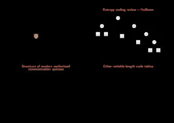
Structure of modern audiovisual communication systems Perceptual Entropy Sensor+ Channel Signal ✲ ✲ ✲ ✲ coding sampling coding coding ❄ Noise Channel ✲ ❄ Perceptual Entropy Channel Human Display ✛ ✛ ✛ ✛ senses decoding decoding decoding 2
Audio-visual lossy coding today typically consists of these steps: → A transducer converts the original stimulus into a voltage. → This analog signal is then sampled and quantized . The digitization parameters (sampling frequency, quantization levels) are preferably chosen generously beyond the ability of human senses or output devices. → The digitized sensor-domain signal is then transformed into a per- ceptual domain . This step often mimics some of the first neural processing steps in humans. → This signal is quantized again, based on a perceptual model of what level of quantization-noise humans can still sense. → The resulting quantized levels may still be highly statistically de- pendent. A prediction or decorrelation transform exploits this and produces a less dependent symbol sequence of lower entropy. → An entropy coder turns that into an apparently-random bit string, whose length approximates the remaining entropy. The first neural processing steps in humans are in effect often a kind of decorrelation transform; our eyes and ears were optimized like any other AV communications system. This allows us to use the same transform for decorrelating and transforming into a perceptually relevant domain. 3
Outline of the remaining four lectures → Quick review of entropy coders for removing redundancy from sequences of statistically independent symbols (Huffman, some commonly used fixed code tables, arithmetic) → Transform coding: techniques for converting sequences of highly- dependent symbols into less-dependent lower-entropy sequences. • run-length coding, fax • decorrelation, Karhunen-Lo` eve transform (Principle Com- ponent Analysis) • other orthogonal transforms (especially DCT) 4
→ Introduction to some characteristics and limits of human senses • perceptual scales (Weber, Fechner, Stevens, dB) and sen- sitivity limits • colour vision • human hearing limits, critical bands, audio masking → Quantization techniques to remove information that is irrele- vant to human senses → Image and audio coding standards • A/ µ -law coding (digital telephone network) • JPEG • MPEG video • MPEG audio 5
Entropy coding review – Huffman 1.00 0 1 0.40 0.60 0 1 0 1 v w 0.25 0.20 0.20 u 0 1 0.35 x 0.10 0.15 0 1 Huffman’s algorithm constructs an optimal code-word tree for a set of symbols with known probability distribution. It iteratively picks the two y z elements of the set with the smallest probability and combines them into 0.05 0.05 a tree by adding a common root. The resulting tree goes back into the set, labeled with the sum of the probabilities of the elements it combines. The algorithm terminates when less than two elements are left. 6
Other variable-length code tables Huffman’s algorithm generates an optimal code table. Disadvantage: this code table (or the distribution from which it was generated) needs to be stored or transmitted. Adaptive variants of Huffman’s algorithm modify the coding tree in the encoder and decoder synchronously, based on the distribution of symbols encountered so far. This enables one-pass processing and avoids the need to transmit or store a code table, at the cost of starting with a less efficient encoding. Unary code Encode the natural number n as the bit string 1 n 0 . This code is optimal when the probability distribution is p ( n ) = 2 − ( n +1) . Example: 3 , 2 , 0 → 1110 , 110 , 0 Golomb code Select an encoding parameter b . Let n be the natural number to be encoded, q = ⌊ n/b ⌋ and r = n − qb . Encode n as the unary code word for q , followed by the ( log 2 b )-bit binary code word for r . Where b is not a power of 2, encode the lower values of r in ⌊ log 2 b ⌋ bits, and the rest in ⌈ log 2 b ⌉ bits, such that the leading digits distinguish the two cases. 7
Examples: b = 1 : 0, 10, 110, 1110, 11110, 111110, . . . (this is just the unary code) b = 2 : 00, 01, 100, 101, 1100, 1101, 11100, 11101, 111100, 111101, . . . b = 3 : 00, 010, 011, 100, 1010, 1011, 1100, 11010, 11011, 11100, 111010, . . . b = 4 : 000, 001, 010, 011, 1000, 1001, 1010, 1011, 11000, 11001, 11010, . . . Golomb codes are optimal for geometric distributions of the form p ( n ) = u n ( u − 1) (e.g., run lengths of Bernoulli experiments) if b is chosen suitably for a given u . S.W. Golomb: Run-length encodings. IEEE Transactions on Information Theory, IT-12(3):399– 401, July 1966. Elias gamma code Start the code word for the positive integer n with a unary-encoded length indicator m = ⌊ log 2 n ⌋ . Then append from the binary notation of n the rightmost m digits (to cut off the leading 1). 1 = 0 4 = 11000 7 = 11011 10 = 1110010 2 = 100 5 = 11001 8 = 1110000 11 = 1110011 3 = 101 6 = 11010 9 = 1110001 . . . P. Elias: Universal codeword sets and representations of the integers. IEEE Transactions on Information Theory, IT-21(2)194–203, March 1975. More such variable-length integer codes are described by Fenwick in IT-48(8)2412–2417, August 2002. (Available on http://ieeexplore.ieee.org/ ) 8
Entropy coding review – arithmetic coding Partition [0,1] according 0.0 0.35 0.55 0.75 0.9 0.95 1.0 to symbol probabilities: u v w x y z Encode text wuvw . . . as numeric value (0.58. . . ) in nested intervals: 1.0 0.75 0.62 0.5885 0.5850 z z z z z y y y y y x x x x x w w w w w v v v v v u u u u u 0.55 0.0 0.55 0.5745 0.5822 9
Arithmetic coding Several advantages: → Length of output bitstring can approximate the theoretical in- formation content of the input to within 1 bit. → Performs well with probabilities > 0.5, where the information per symbol is less than one bit. → Interval arithmetic makes it easy to change symbol probabilities (no need to modify code-word tree) ⇒ convenient for adaptive coding Can be implemented efficiently with fixed-length arithmetic by rounding probabilities and shifting out leading digits as soon as leading zeros appear in interval size. Usually combined with adaptive probability estimation. Huffman coding remains popular because of its simplicity and lack of patent-licence issues. 10
Coding of sources with memory and correlated symbols Run-length coding: ↓ 5 7 12 3 3 Predictive coding: encoder decoder f(t) g(t) g(t) f(t) − + predictor predictor P(f(t−1), f(t−2), ...) P(f(t−1), f(t−2), ...) Delta coding (DPCM): P ( x ) = x n � Linear predictive coding: P ( x 1 , . . . , x n ) = a i x i i =1 11
Old (Group 3 MH) fax code pixels white code black code • Run-length encoding plus modified Huffman 0 00110101 0000110111 code 1 000111 010 2 0111 11 • Fixed code table (from eight sample pages) 3 1000 10 • separate codes for runs of white and black 4 1011 011 pixels 5 1100 0011 • termination code in the range 0–63 switches 6 1110 0010 between black and white code 7 1111 00011 8 10011 000101 • makeup code can extend length of a run by 9 10100 000100 a multiple of 64 10 00111 0000100 • termination run length 0 needed where run 11 01000 0000101 length is a multiple of 64 12 001000 0000111 • single white column added on left side be- 13 000011 00000100 fore transmission 14 110100 00000111 • makeup codes above 1728 equal for black 15 110101 000011000 and white 16 101010 0000010111 . . . . . . . . . • 12-bit end-of-line marker: 000000000001 63 00110100 000001100111 (can be prefixed by up to seven zero-bits 64 11011 0000001111 to reach next byte boundary) 128 10010 000011001000 Example: line with 2 w, 4 b, 200 w, 3 b, EOL → 192 010111 000011001001 1000 | 011 | 010111 | 10011 | 10 | 000000000001 . . . . . . . . . 1728 010011011 0000001100101 12
Modern (JBIG) fax code Performs context-sensitive arithmetic coding of binary pixels. Both encoder and decoder maintain statistics on how the black/white prob- ability of each pixel depends on these 10 previously transmitted neigh- bours: ? Based on the counted numbers n black and n white of how often each pixel value has been encountered so far in each of the 1024 contexts, the probability for the next pixel being black is estimated as n black + 1 p black = n white + n black + 2 The encoder updates its estimate only after the newly counted pixel has been encoded, such that the decoder knows the exact same statistics. Joint Bi-level Expert Group: International Standard ISO 11544, 1993. Example implementation: http://www.cl.cam.ac.uk/~mgk25/jbigkit/ 13
Recommend
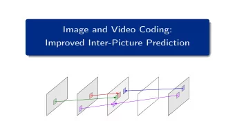
![Image and Video Coding: Hybrid Video Coding s n 1 [ x , y ] s n [ x , y ] m k = ( m x , m](https://c.sambuz.com/761427/image-and-video-coding-hybrid-video-coding-s.webp)

![Image and Video Coding: Video Coding Standards s k [ x , y ] u k [ x , y ] quantization indexes q](https://c.sambuz.com/892752/image-and-video-coding-video-coding-standards-s.webp)

More recommend
Explore More Topics
Stay informed with curated content and fresh updates.