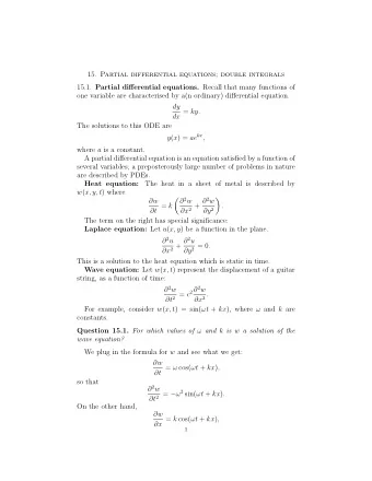
INF5620: Numerical Methods for Partial Differential Equations Hans - - PowerPoint PPT Presentation

5mm.

INF5620: Numerical Methods for Partial Differential Equations

Hans Petter Langtangen Simula Research Laboratory, and

• Dept. of Informatics, Univ. of Oslo

Last update: April 29, 2011

INF5620: Numerical Methods for Partial Differential Equations – p.1/148

Nonlinear PDEs

Nonlinear PDEs – p.2/148

Examples

Some nonlinear model problems to be treated next: −u′′(x) = f(u), u(0) = uL, u(1) = uR, −(α(u)u′)′ = 0, u(0) = uL, u(1) = uR −∇ · [α(u)∇u] = g(x), with u or − α∂u ∂n B.C. Discretization methods: standard finite difference methods standard finite element methods the group finite element method We get nonlinear algebraic equations Solution method: iterate over linear equations

Nonlinear PDEs – p.3/148

Nonlinear discrete equations; FDM

Finite differences for −u′′ = f(u): − 1 h2 (ui−1 − 2ui + ui+1) = f(ui) ⇒ nonlinear system of algebraic equations F (u) = 0, or Au = b(u), u = (u0, . . . , uN)T Finite differences for (α(u)u′)′ = 0: 1 h2 (α(ui+1/2)(ui+1 − ui) − α(ui−1/2)(ui − ui−1)) = 0 1 2h2 ([α(ui+1)+α(ui)](ui+1 −ui)−[α(ui)+α(ui−1)](ui −ui−1)) = 0 ⇒ nonlinear system of algebraic equations F (u) = 0

• r

A(u)u = b

Nonlinear PDEs – p.4/148

Nonlinear discrete equations; FEM

Finite elements for −u′′ = f(u) with u(0) = u(1) = 0 Galerkin approach: find u = n

k=1 ukϕk(x) ∈ V such that

1 u′v′dx = 1 f(u)vdx ∀v ∈ V Left-hand side is easy to assemble: v = ϕi − 1 h (ui−1 − 2ui + ui+1) = 1 f(

• k

ukϕk(x))ϕidx We write u =

k ukϕk instead of u = k ckϕk since

ck = u(xk) = uk and uk is used in the finite difference schemes

Nonlinear PDEs – p.5/148

Nonlinearities in the FEM

Note that f(

• k

ϕk(x)uk) is a complicated function of u0, . . . , uN F .ex.: f(u) = u2 1

• k

ϕkuk 2 ϕidx gives rise to a difference representation h 12

• u2

i−1 + 2ui(ui−1 + ui+1) + 6u2 i + u2 i+1

• (compare with f(ui) = u2

i in FDM!)

Must use numerical integration in general to evaluate

• f(u)ϕidx

Nonlinear PDEs – p.6/148

The group finite element method

The group finite element method: f(u) = f(

• j

ujϕj(x)) ≈

n

• j=1

f(uj)ϕj Resulting term: 1

0 f(u)ϕidx =

1

• j ϕiϕjf(uj) gives
• j

1 ϕkϕidx

• f(uj)

This integral and formulation also arise from approxmating some function by u =

j ujϕj

We can write the term as Mf(u), where M has rows consisting

• f h/6(1, 4, 1), and row i in Mf(u) becomes

h 6 (f(ui−1) + 4f(ui) + f(ui+1))

Nonlinear PDEs – p.7/148

FEM for a nonlinear coefficient

We now look at (α(u)u′)′ = 0, u(0) = uL, u(1) = uR Using a finite element method (fine exercise!) results in an integral 1 α(

• k

ukϕk)ϕ′

iϕ′ j dx

⇒ complicated to integrate by hand or symbolically Linear P1 elements and trapezoidal rule (do it!): 1 2(α(ui) + α(ui+1))(ui+1 − ui) − 1 2(α(ui−1) + α(ui))(ui − ui−1) = 0 ⇒ same as FDM with arithmetic mean for α(ui+1/2)

Nonlinear PDEs – p.8/148

Nonlinear algebraic equations

FEM/FDM for nonlinear PDEs gives nonlinear algebraic equations: (α(u)u′)′ = 0 ⇒ A(u)u = b −u′′ = f(u) ⇒ Au = b(u) In general a nonlinear PDE gives F (u) = 0

• r

F0(u0, . . . , uN) = . . . FN(u0, . . . , uN) =

Nonlinear PDEs – p.9/148

Solving nonlinear algebraic eqs.

Have A(u)u − b = 0, Au − b(u) = 0, F (u) = 0 Idea: solve nonlinear problem as a sequence of linear subproblems Must perform some kind of linearization Iterative method: guess u0, solve linear problems for u1, u2, . . . and hope that lim

q→∞ uq = u

i.e. the iteration converges

Nonlinear PDEs – p.10/148

Picard iteration (1)

Model problem: A(u)u = b Simple iteration scheme: A(uq)uq+1 = b, q = 0, 1, . . . Must provide (good) guess u0 Termination: ||uq+1 − uq|| ≤ ǫu

• r using the residual (expensive, req. new A(uq+1)!)

||b − A(uq+1)uq+1|| ≤ ǫr Relative criteria: ||uq+1 − uq|| ≤ ǫu||uq||

• r (more expensive)

||b − A(uq+1)uq+1|| ≤ ǫr||b − A(u0)u0||

Nonlinear PDEs – p.11/148

Picard iteration (2)

Model problem: Au = b(u) Simple iteration scheme: Auq+1 = b(uq), q = 0, 1, . . . Relaxation: Au∗ = b(uq), uq+1 = ωu∗ + (1 − ω)uq (may improve convergence, avoids too large steps) This method is also called Successive substitutions

Nonlinear PDEs – p.12/148

Newton’s method for scalar equations

The Newton method for f(x) = 0, x ∈ I R Given an approximation xq Approximate f by a linear function at xq: f(x) ≈ M(x; xq) = f(xq) + f ′(xq)(x − xq) Find new xq+1 such that M(xq+1; xq) = 0 ⇒ xq+1 = xq − f(xq) f ′(xq)

Nonlinear PDEs – p.13/148

Newton’s method for systems of equations

Systems of nonlinear equations: F (u) = 0, F (u) ≈ M(u; uq) Multi-dimensional Taylor-series expansion: M(u; uq) = F (uq) + J(u − uq), J ≡ ∇F Ji,j = ∂Fi ∂uj Iteration no. q: solve linear system J(uq)(δu)q+1 = −F (uq) update: uq+1 = uq + (δu)q+1 Can use relaxation: uq+1 = uq + ω(δu)q+1

Nonlinear PDEs – p.14/148

The Jacobian matrix; FDM (1)

Model equation: u′′ = −f(u) Scheme: Fi ≡ 1 h2 (ui−1 − 2ui + ui+1) + f(ui) = 0 Jacobian matrix term (FDM): Ji,j = ∂Fi ∂uj Fi contains only ui, ui±1 Only Ji,i−1 = ∂Fi ∂ui−1 , Ji,i = ∂Fi ∂ui , Ji,i+1 = ∂Fi ∂ui+1 = 0 ⇒ Jacobian is tridiagonal

Nonlinear PDEs – p.15/148

The Jacobian matrix; FDM (2)

Fi ≡ 1 h2 (ui−1 − 2ui + ui+1) − f(ui) = 0 Derivation: Ji,i−1 = ∂Fi ∂ui−1 = 1 h2 Ji,i+1 = ∂Fi ∂ui+1 = 1 h2 Ji,i = ∂Fi ∂ui = − 2 h2 + f ′(ui) Must form the Jacobian matrix J in each iteration and solve Jδuq+1 = −F (uq) and then update uq+1 = uq + ωδuq+1

Nonlinear PDEs – p.16/148

The Jacobian matrix; FEM

−u′′ = f(u) on Ω = (0, 1) with u(0) = u(1) = 0 and FEM Fi ≡ 1

• k

ϕ′

iϕ′ kuk − f(

• s

usϕs)ϕi

• dx = 0

First term of the Jacobian Ji,j = ∂Fi

∂uj :

∂ ∂uj 1

• k

ϕ′

iϕ′ kuk dx =

1 ∂ ∂uj

• k

ϕ′

iϕ′ kuk dx =

1 ϕ′

iϕ′ j dx

Second term: − ∂ ∂uj 1 f(

• s

usϕs)ϕi dx = − 1 f ′(

• s

usϕs)ϕjϕi dx because when u =

s usϕs, ∂ ∂uj f(u) = f ′(u) ∂u ∂uj = f ′(u) ∂ ∂uj

• s usϕs = f ′(u)ϕj

Nonlinear PDEs – p.17/148

A 2D/3D transient nonlinear PDE (1)

PDE for heat conduction in a solid where the conduction depends

• n the temperature u:

̺C ∂u ∂t = ∇ · [κ(u)∇u] (f.ex. u = g on the boundary and u = I at t = 0) Stable Backward Euler FDM in time: un − un−1 ∆t = ∇ · [α(un)∇un] with α = κ/(̺C) Next step: Galerkin formulation, where un =

j un j ϕj is the

unknown and un−1 is just a known function

Nonlinear PDEs – p.18/148

A 2D/3D transient nonlinear PDE (2)

FEM gives nonlinear algebraic equations: Fi(un

0, . . . , un N) = 0,

i = 0, . . . , N where Fi ≡

• Ω
• un − un−1

v + ∆tα(un)∇un · ∇v

• dΩ

Nonlinear PDEs – p.19/148

A 2D/3D transient nonlinear PDE (3)

Picard iteration: Use “old” un,q in α(un) term, solve linear problem for un,q+1, q = 0, 1, . . . Ai,j =

• Ω

(ϕiϕj + ∆tα(un,q)∇ϕi · ∇ϕj) dΩ bi =

• Ω

un−1ϕidΩ Newton’s method: need Jacobian, Ji,j = ∂Fi ∂un

j

Ji,j =

• Ω

(ϕiϕj + ∆t(α′(un,q)ϕj∇un,q · ∇ϕi + α(un,q)∇ϕi · ∇ϕj)) dΩ

Nonlinear PDEs – p.20/148

Iteration methods at the PDE level

Consider −u′′ = f(u) Could introduce Picard iteration at the PDE level: − d2 dx2 uq+1 = f(uq), q = 0, 1, . . . ⇒ linear problem for uq+1 A PDE-level Newton method can also be formulated (see the HPL book for details) We get identical results for our model problem Time-dependent problems: first use finite differences in time, then use an iteration method (Picard or Newton) at the time-discrete PDE level

Nonlinear PDEs – p.21/148

Continuation methods

Challenging nonlinear PDE: ∇ · (||∇u||q∇u) = 0 For q = 0 this problem is simple Idea: solve a sequence of problems, starting with q = 0, and increase q towards a target value Sequence of PDEs: ∇ · (||∇ur||qr∇ur) = 0, r = 0, 1, 2, . . . with = 0 < q0 < q1 < q2 < · · · < qm = q Start guess for ur is ur−1 (the solution of a “simpler” problem) CFD: The Reynolds number is often the continuation parameter q

Nonlinear PDEs – p.22/148

Exercise 1

Derive the nonlinear algebraic equations for the problem d dx

• α(u)du

dx

• = 0 on (0, 1),

u(0) = 0, u(1) = 1, using a finite difference method and the Galerkin method with P1 finite elements and the Trapezoidal rule for approximating integrals.

Nonlinear PDEs – p.23/148

Exercise 2

For the problem in Exercise 1, use the group finite element method with P1 elements and the Trapezoidal rule for integrals and show that the resulting equations coincide with those

• btained in Exercise 1.

Nonlinear PDEs – p.24/148

Exercise 3

For the problem in Exercises 1 and 2, identify the F vector in the system F = 0 of nonlinear equations. Derive the Jacobian J for a general α(u). Then write the expressions for the Jacobian when α(u) = α0 + α1u + α2u2.

Nonlinear PDEs – p.25/148

Exercise 4

Explain why discretization of nonlinear differential equations by finite difference and finite element methods normally leads to a Jacobian with the same sparsity pattern as one would encounter in an associated linear problem. Hint: Which unknowns will enter equation number i?

Nonlinear PDEs – p.26/148

Exercise 5

Show that if F (u) = 0 is a linear system of equations, F = Au − b, for a constant matrix A and vector b, then Newton’s method (with ω = 1) finds the correct solution in the first iteration.

Nonlinear PDEs – p.27/148

Exercise 6

The operator ∇ · (α∇u), with α = ||∇u||q, q ∈ I R, and || · || being the Eucledian norm, appears in several physical problems, especially flow of non-Newtonian fluids. The quantity ∂α/∂uj is central when formulating a Newton method, where uj is the coefficient in the finite element approximation u =

j ujϕj. Show

that ∂ ∂uj ||∇u||q = q||∇u||q−2∇u · ∇ϕj .

Nonlinear PDEs – p.28/148

Exercise 7

Consider the PDE ∂u ∂t = ∇ · (α(u)∇u) discretized by a Forward Euler difference in time. Explain why this nonlinear PDE gives rise to a linear problem (and hence no need for Newton or Picard iteration) at each time level. Discretize the PDE by a Backward Euler difference in time and realize that there is a need for solving nonlinear algebraic

• equations. Formulate a Picard iteration method for the spatial

PDE to be solved at each time level. Formulate a Galerkin method for discretizing the spatial problem at each time level. Choose some appropriate boundary conditions. Explain how to incorporate an initial condition.

Nonlinear PDEs – p.29/148

Exercise 8

Repeat Exercise 7 for the PDE ̺(u)∂u ∂t = ∇ · (α(u)∇u)

Nonlinear PDEs – p.30/148

Exercise 9

For the problem in Exercise 8, assume that a nonlinear Newton cooling law applies at the whole boundary: −α(u)∂u ∂n = H(u)(u − uS), where H(u) is a nonlinear heat transfer coefficient and uS is the temperature of the surroundings (and u is the temperature). Use a Backward Euler scheme in time and a Galerkin method in space. Identify the nonlinear algebraic equations to be solved at each time level. Derive the corresponding Jacobian. The PDE problem in this exercise is highly relevant when the temperature variations are large. Then the density times the heat capacity (̺), the heat conduction coefficient (α) and the heat transfer coefficient (H) normally vary with the temperature (u).

Nonlinear PDEs – p.31/148

Exercise 10

In Exercise 8, restrict the problem to one space dimension, choose simple boundary conditions like u = 0, use the group finite element method for all nonlinear coefficients, apply P1 elements, use the Trapezoidal rule for all integrals, and derive the system of nonlinear algebraic equations that must be solved at each time level. Set up some finite difference method and compare the form of the nonlinear algebraic equations.

Nonlinear PDEs – p.32/148

Exercise 11

In Exercise 8, use the Picard iteration method with one iteration at each time level, and introduce this method at the PDE level. Realize the similarities with the resulting discretization and that of the corresponding linear diffusion problem.

Nonlinear PDEs – p.33/148

Shallow water waves

Shallow water waves – p.34/148

Tsunamis

Waves in fjords, lakes, or oceans, generated by slide earthquake subsea volcano asteroid human activity, like nuclear detonation, or slides generated by oil drilling, may generate tsunamis Propagation over large distances Hardly recognizable in the open ocean, but wave amplitude increases near shore Run-up at the coasts may result in severe damage Giant events: Dec 26 2004 (≈ 300000 killed), 1883 (similar to 2004), 65 My ago (extinction of the dinosaurs)

Shallow water waves – p.35/148

Norwegian tsunamis

5 ˚ 1 ˚ 1 5 ˚ 6 ˚ 6 5 ˚ 70˚

Oslo Stockholm

Bergen Tromsø Bodø Trondheim

N O R W A Y S W E D E N

Circules: Major incidents, > 10 killed; Triangles: Selected smaller incidents; Square: Storegga (5000 B.C.)

Shallow water waves – p.36/148

Tsunamis in the Pacific

Scenario: earthquake outside Chile, generates tsunami, propagating at 800 km/h accross the Pacific, run-up on densly populated coasts in Japan;

Shallow water waves – p.37/148

Selected events; slides

location year run-up dead Loen 1905 40m 61 Tafjord 1934 62m 41 Loen 1936 74m 73 Storegga 5000 B.C. 10m(?) ?? Vaiont, Italy 1963 270m 2600 Litua Bay, Alaska 1958 520m 2 Shimabara, Japan 1792 10m(?) 15000

Shallow water waves – p.38/148

Selected events; earthquakes etc.

location year strength run-up dead Thera 1640 B.C. volcano ? ? Thera 1650 volcano ? ? Lisboa 1755 M=9 ? 15(?)m ?000 Portugal 1969 M=7.9 1 m Amorgos 1956 M=7.4 5(?)m 1 Krakatao 1883 volcano 40 m 36 000 Flores 1992 M=7.5 25 m 1 000 Nicaragua 1992 M=7.2 10 m 168 Sumatra 2004 M=9 50 m 300 000 The selection is biased wrt. European events; 150 catastrophic tsunami events have been recorded along along the Japanese coast in modern times. Tsunamis: no. 5 killer among natural hazards

Shallow water waves – p.39/148

Why simulation?

Increase the understanding of tsunamis Assist warning systems Assist building of harbor protection (break waters) Recognize critical coastal areas (e.g. move population) Hindcast historical tsunamis (assist geologists/biologists)

Shallow water waves – p.40/148

Problem sketch

η(x,y,t) y z x H(x,y,t)

Assume wavelength ≫ depth (long waves) Assume small amplitudes relative to depth Appropriate approx. for many ocean wave phenomena Reference: HPL chapter 6.2

Shallow water waves – p.41/148

Mathematical model

PDEs: ∂η ∂t = − ∂ ∂x (uH) − ∂ ∂y (vH)

• −∂H

∂t

• ∂u

∂t = −∂η ∂x, x ∈ Ω, t > 0 ∂v ∂t = −∂η ∂y , x ∈ Ω, t > 0 η(x, y, t) : surface elevation u(x, y, t) and v(x, y, t) : horizontal (depth averaged) velocities H(x, y) : stillwater depth (given) Boundary conditions: either η, u or v given at each point Initial conditions: all of η, u and v given

Shallow water waves – p.42/148

Primary unknowns

Discretization: finite differences Staggered mesh in time and space ⇒ η, u, and v unknown at different points: ηℓ

i+ 1

2 ,j+ 1 2 ,

u

ℓ+ 1

2

i,j+ 1

2 ,

v

ℓ+ 1

2

i+ 1

2 ,j+1

r ηℓ

i+ 1

2 ,j+ 1 2

u

ℓ+ 1

2

i,j+ 1

2

u

ℓ+ 1

2

i+1,j+ 1

2

v

ℓ+ 1

2

i+ 1

2 ,j

v

ℓ+ 1

2

i+ 1

2 ,j+1

Shallow water waves – p.43/148

A global staggered mesh

Widely used mesh in computational fluid dynamics (CFD) Important for Navier-Stokes solvers Basic idea: centered differences in time and space

Shallow water waves – p.44/148

Discrete equations; η

∂η ∂t = − ∂ ∂x (uH) − ∂ ∂y (vH) at (i + 1 2, j + 1 2, ℓ − 1 2) [Dtη = −Dx(uH) − Dy(vH)]

ℓ− 1

2

i+ 1

2 ,j+ 1 2

1 ∆t

• ηℓ

i+ 1

2 ,j+ 1 2 − ηℓ−1

i+ 1

2 ,j+ 1 2

• =

− 1 ∆x

• (Hu)

ℓ− 1

2

i+1,j+ 1

2 − (Hu)

ℓ− 1

2

i,j+ 1

2

• − 1

∆y

• (Hv)

ℓ− 1

2

i+ 1

2 ,j+1 − (Hv)

ℓ− 1

2

i+ 1

2 ,j

• Shallow water waves – p.45/148

Discrete equations; u

∂u ∂t = −∂η ∂x at (i, j + 1 2, ℓ) [Dtu = −Dxη]ℓ

i,j+ 1

2

1 ∆t

• u

ℓ+ 1

2

i,j+ 1

2 − u

ℓ− 1

2

i,j+ 1

2

• =

− 1 ∆x

• ηℓ

i+ 1

2 ,j+ 1 2 − ηℓ

i− 1

2 ,j+ 1 2

• Shallow water waves – p.46/148

Discrete equations; v

∂v ∂t = −∂η ∂y at (i + 1 2, j, ℓ) [Dtv = −Dyη]ℓ

i+ 1

2,j

1 ∆t

• v

ℓ+ 1

2

i+ 1

2 ,j − v

ℓ− 1

2

i+ 1

2 ,j

• =

1 ∆y

• ηℓ

i+ 1

2 ,j+ 1 2 − ηℓ

i+ 1

2 ,j− 1 2

• Shallow water waves – p.47/148

Complicated costline boundary

Saw-tooth approximation to real boundary Successful method, widely used Warning: can lead to nonphysical waves

Shallow water waves – p.48/148

Relation to the wave equation

Eliminate u and v (easy in the PDEs) and get ∂2η ∂t2 = ∇ · [H(x, y)∇η] Eliminate discrete u and v ⇒ Standard 5-point explicit finite difference scheme for discrete η (quite some algebra needed, try 1D first)

Shallow water waves – p.49/148

Stability and accuracy

Centered differences in time and space Truncation error, dispersion analysis: O(∆x2, ∆y2, ∆t2) Stability as for the std. wave equation in 2D: ∆t ≤ H− 1

2

• 1

1 ∆x2 + 1 ∆y2

(CFL condition) If H const, exact numerical solution is possible for

• ne-dimensional wave propagation

Shallow water waves – p.50/148

Verification of an implementation

How can we verify that the program works? Compare with an analytical solution (if possible) Check that basic physical mechanisms are reproduced in a qualitatively correct way by the program

Shallow water waves – p.51/148

Tsunami due to a slide

Surface elevation ahead of the slide, dump behind Initially, negative dump propagates backwards The surface waves propagate faster than the slide moves

Shallow water waves – p.52/148

Tsunami due to faulting

The sea surface deformation reflect the bottom deformation Velocity of surface waves (H ∼ 5 km): 790 km/h Velocity of seismic waves in the bottom: 6000–25000 km/h

Shallow water waves – p.53/148

Tsunami approaching the shore

The velocity of a tsunami is

• gH(x, y, t).

The back part of the wave moves at higher speed ⇒ the wave becomes more peak-formed Deep water (H ∼ 3 km): wave length 40 km, height 1 m Shallow water (H ∼ 10 m): wave length 2 km, height 4 m

Shallow water waves – p.54/148

Tsunamis experienced from shore

As a fast tide, with strong currents in fjords A wall of water approaching the beach Wave breaking: the top has larger effective depth and moves faster than the front part (requires a nonlinear PDE)

Shallow water waves – p.55/148

Convection-dominated flow

Convection-dominated flow – p.56/148

Typical transport PDE

Transport of a scalar u (heat, pollution, ...) in fluid flow v: ∂u ∂t + v · ∇u = α∇2u + f Convection (change of u due to the flow): v · ∇u Diffusion (change of u due to molecular collisions): α∇2u Common case: convection ≫ diffusion → numerical difficulties Important dimensionless number: Peclet number Pe Pe = |v · ∇u| |α∇2u| ∼ V U/L αU/L2 = V L α V : characteristic velocity v, L: characteristic length scale, α: diffusion constant, U: characteristic size of u

Convection-dominated flow – p.57/148

The transport PDE for fluid flow

The fluid flow itself is governed by Navier-Stokes equations: ∂v ∂t + v · v = −1 ̺∇p + ν∇2v + f ∇ · v = 0 Important dimensionless number: Reynolds number Re Re = convection diffusion = |v · ∇v| |ν∇2v| ∼ V 2/L αV/L2 = V L ν Re ≫ 1 and Pe ≫ 1: numerical difficulties

Convection-dominated flow – p.58/148

A 1D stationary transport problem

Assumption: no time, 1D, no source term v · ∇u = α∇2u → vu′ = αu′′ → u′ = ǫu′′, ǫ = α v Complete model problem: u′(x) = ǫu′′(x), x ∈ (0, 1), u(0) = 0, u(1) = 1 ǫ small: boundary layer at x = 1 Standard numerics (i.e. centered differences) will fail! Cure: upwind differences

Convection-dominated flow – p.59/148

Notation for difference equations (1)

Define [Dxu]n

i,j,k ≡

un

i+ 1

2 ,j,k − un

i− 1

2 ,j,k

h with similar definitions of Dy, Dz, and Dt Another difference: [D2xu]n

i,j,k ≡

un

i+1,j,k − un i−1,j,k

2h Compound difference: [DxDxu]n

i = 1

h2

• un

i−1 − 2un i + un i+1

• Convection-dominated flow – p.60/148

Notation for difference equations (1)

One-sided forward difference: [D+

x u]n i ≡ un i+1 − un i

h and the backward difference: [D−

x u]n i ≡ un i − un i−1

h Put the whole equation inside brackets: [DxDxu = −f]i is a finite difference scheme for u′′ = −f

Convection-dominated flow – p.61/148

Centered differences

u′(x) = ǫu′′(x), x ∈ (0, 1), u(0) = 0, u(1) = 1 ui+1 − ui−1 2h = ǫui−1 − 2ui + ui+1 h2 , i = 2, . . . , n − 1 u1 = 0, un = 1

• r

[D2xu = ǫDxDxu]i Analytical solution: u(x) = 1 − ex/ǫ 1 − e1/ǫ ⇒ u′(x) > 0, i.e., monotone function

Convection-dominated flow – p.62/148

Numerical experiments (1)

• 0.8
• 0.6
• 0.4
• 0.2

0.2 0.4 0.6 0.8 1 1.2 0.2 0.4 0.6 0.8 1 u(x) x n=20, epsilon=0.1 centered exact

Convection-dominated flow – p.63/148

Numerical experiments (2)

• 0.8
• 0.6
• 0.4
• 0.2

0.2 0.4 0.6 0.8 1 1.2 0.2 0.4 0.6 0.8 1 u(x) x n=20, epsilon=0.01 centered exact

Convection-dominated flow – p.64/148

Numerical experiments (3)

• 0.8
• 0.6
• 0.4
• 0.2

0.2 0.4 0.6 0.8 1 1.2 0.2 0.4 0.6 0.8 1 u(x) x n=80, epsilon=0.01 centered exact

Convection-dominated flow – p.65/148

Numerical experiments (4)

• 0.8
• 0.6
• 0.4
• 0.2

0.2 0.4 0.6 0.8 1 1.2 0.2 0.4 0.6 0.8 1 u(x) x n=20, epsilon=0.001 centered exact

Convection-dominated flow – p.66/148

Numerical experiments; summary

The solution is not monotone if h > 2ǫ The convergence rate is h2 (expected since both differences are of 2nd order) provided h ≤ 2ǫ Completely wrong qualitative behavior for h ≫ 2ǫ

Convection-dominated flow – p.67/148

Analysis

Can find an analytical solution of the discrete problem (!) Method: insert ui ∼ βi and solve for β β1 = 1, β2 = 1 + h/(2ǫ) 1 − h/(2ǫ)

• cf. HPL app. A.4.4

Complete solution: ui = C1βi

1 + C2βi 2

Determine C1 and C2 from boundary conditions ui = βi

2 − β2

βn

2 − β2

Convection-dominated flow – p.68/148

Important result

Observe: ui oscillates if β2 < 0 ⇒ 1 + h/(2ǫ) 1 − h/(2ǫ) < 0 ⇒ h > 2ǫ Must require h ≤ 2ǫ for ui to have the same qualitative property as u(x) This explains why we observed oscillations in the numerical solution

Convection-dominated flow – p.69/148

Upwind differences

Problem: u′(x) = ǫu′′(x), x ∈ (0, 1), u(0) = 0, u(1) = 1 Use a backward difference, called upwind difference, for the u′ term: ui − ui−1 h = ǫui−1 − 2ui + ui+1 h2 , i = 2, . . . , n − 1 u1 = 0, un = 1 The scheme can be written as [D−

x u = ǫDxDxu]i

Convection-dominated flow – p.70/148

Numerical experiments (1)

• 0.8
• 0.6
• 0.4
• 0.2

0.2 0.4 0.6 0.8 1 1.2 0.2 0.4 0.6 0.8 1 u(x) x n=20, epsilon=0.1 upwind exact

Convection-dominated flow – p.71/148

Numerical experiments (2)

• 0.8
• 0.6
• 0.4
• 0.2

0.2 0.4 0.6 0.8 1 1.2 0.2 0.4 0.6 0.8 1 u(x) x n=20, epsilon=0.01 upwind exact

Convection-dominated flow – p.72/148

Numerical experiments; summary

The solution is always monotone, i.e., always qualitatively correct The boundary layer is too thick The convergence rate is h (in agreement with truncation error analysis)

Convection-dominated flow – p.73/148

Analysis

Analytical solution of the discrete equations: ui = βi ⇒ β1 = 1, β2 = 1 + h/ǫ ui = C1 + C2βi

2

Using boundary conditions: ui = βi

2 − β2

βn

2 − β2

Since β2 > 0 (actually β2 > 1), βi

2 does not oscillate

Convection-dominated flow – p.74/148

Centered vs. upwind scheme

Truncation error: centered is more accurate than upwind Exact analysis: centered is more accurate than upwind when centered is stable (i.e. monotone ui), but otherwise useless ǫ = 10−6 ⇒ 500 000 grid points to make h ≤ 2ǫ Upwind gives best reliability, at a cost of a too thick boundary layer

Convection-dominated flow – p.75/148

An interpretation of the upwind scheme

The upwind scheme ui − ui−1 h = ǫui−1 − 2ui + ui+1 h2

• r

[D−

x u = ǫDxDxu]i

can be rewritten as ui+1 − ui−1 2h = (ǫ + h 2 )ui−1 − 2ui + ui+1 h2

• r

[D2xu = (ǫ + h 2 )DxDxu]i Upwind = centered + artificial diffusion (h/2)

Convection-dominated flow – p.76/148

Finite elements for the model problem

Galerkin formulation of u′(x) = ǫu′′(x), x ∈ (0, 1), u(0) = 0, u(1) = 1 and linear (P1) elements leads to a centered scheme (show it!) ui+1 − ui−1 2h = ǫui−1 − 2ui + ui+1 h2 , i = 2, . . . , n − 1 u1 = 0, un = 1

• r

[D2xu = ǫDxDxu]i Stability problems when h > 2ǫ

Convection-dominated flow – p.77/148

Finite elements and upwind differences

How to construct upwind differences in a finite element context? One possibility: add artificial diffusion (h/2) u′(x) = (ǫ + h 2 )u′′(x), x ∈ (0, 1), u(0) = 0, u(1) = 1 Can be solved by a Galerkin method Another, equivalent strategy: use of perturbed weighting functions

Convection-dominated flow – p.78/148

Perturbed weighting functions in 1D

Take wi(x) = ϕi(x) + τϕ′

i(x)

• r alternatively written

w(x) = v(x) + τv′(x) where v is the standard test function in a Galerkin method Use this wi or w as test function for the convective term u′: 1 u′wdx = 1 u′vdx + 1 τu′v′dx The new term τu′v′ is the weak formulation of an artificial diffusion term τu′′v With τ = h/2 we then get the upwind scheme

Convection-dominated flow – p.79/148

Optimal artificial diffusion

Try a weighted sum of a centered and an upwind discretization: [u′]i ≈ [θD−

x u + (1 − θ)D2xu]i,

0 ≤ θ ≤ 1 [θD−

x u + (1 − θ)D2xu = ǫDxDxu]i

Is there an optimal θ? Yes, for θ(h/ǫ) = coth h 2ǫ − 2ǫ h we get exact ui (i.e. u exact at nodal points) Equivalent artificial diffusion τo = 0.5hθ(h/ǫ) Exact finite element method: w(x) = v(x) + τov′(x) for the convective term u′

Convection-dominated flow – p.80/148

Multi-dimensional problems

Model problem: v · ∇u = α∇2u

• r written out:

vx ∂u ∂x + vy ∂u ∂y = α∇2u Non-physical oscillations occur with centered differences or Galerkin methods when the left-hand side terms are large Remedy: upwind differences Downside: too much diffusion Important result: extra stabilizing diffusion is needed only in the streamline direction, i.e., in the direction of v = (vx, vy)

Convection-dominated flow – p.81/148

Streamline diffusion

Idea: add diffusion in the streamline direction Isotropic physical diffusion, expressed through a diffusion tensor:

d

• i=1

d

• j=1

αδij ∂2u ∂xi∂xj = α∇2u αδij is the diffusion tensor (here: same in all directions) Streamline diffusion makes use of an anisotropic diffusion tensor αij:

d

• i=1

d

• j=1

∂ ∂xi

• αij

∂u ∂xj

• ,

αij = τ vivj ||v||2 Implementation: artificial diffusion term or perturbed weighting function

Convection-dominated flow – p.82/148

Perturbed weighting functions (1)

Consider the weighting function w = v + τ ∗v · ∇v for the convective (left-hand side) term:

• w v · ∇u dΩ

This expands to

• vv · ∇udΩ +
• τ ∗v · ∇u v · ∇vdΩ

The latter term can be viewed as the Galerkin formulation of (write v · ∇u =

i ∂u/∂xi etc.) d

• i=1

d

• j=1

∂ ∂xi

• τ ∗vivj

∂u ∂xj

• Convection-dominated flow – p.83/148

Perturbed weighting functions (2)

⇒ Streamline diffusion can be obtained by perturbing the weighting function Common name: SUPG (streamline-upwind/Petrov-Galerkin)

Convection-dominated flow – p.84/148

Consistent SUPG

Why not just add artificial diffusion? Why bother with perturbed weighting functions? In standard FEM (method of weighted residuals),

• Ω

L(u)wΩ = 0 the exact solution is a solution of the FEM equations (it fulfills L(u)) This no longer holds if we add an artificial diffusion term (∼ h/2) use different weighting functions on different terms Idea: use consistent SUPG no artificial diffusion term same (perturbed) weighting function applies to all terms

Convection-dominated flow – p.85/148

A step back to 1D

Let us try to use w(x) = v(x) + τv′(x)

• n both terms in u′ = ǫu′′:

1 (u′v + (ǫ + τ)u′v′)dx + τ 1 v′′u′dx = 0 Problem: last term contains v′′ Remedy: drop it (!) Justification: v′′ = 0 on each linear (P1) element Drop 2nd-order derivatives of v in 2D/3D too Consistent SUPG is not so consistent...

Convection-dominated flow – p.86/148

Choosing τ ∗

Choosing τ ∗ is a research topic Many suggestions Two classes: τ ∗ ∼ h τ ∗ ∼ ∆t (time-dep. problems) Little theory

Convection-dominated flow – p.87/148

A test problem (1)

u=0 u=0 du/dn=0

• r

1 1 y x u=1 θ v

y = x tan θ + 0.25

0.25 u=0 du/dn=0

Convection-dominated flow – p.88/148

A test problem (2)

Methods:

• 1. Classical SUPG:

Brooks and Hughes: "A streamline upwind/Petrov-Galerkin finite element formulation for advection domainated flows with particular emphasis on the incompressible Navier-Stokes equations", Comp. Methods Appl. Mech. Engrg., 199-259, 1982.

• 2. An additional discontinuity-capturing term

w = v + τ ∗v · ∇v + ˆ τ v · ∇u ||∇u||2 ∇u was proposed in Hughes, Mallet and Mizukami: "A new finite element formulation for computational fluid dynamics: II. Beyond SUPG", Comp. Methods Appl. Mech. Engrg., 341-355, 1986.

Convection-dominated flow – p.89/148

Galerkin’s method

X Y Z −0.65 1 2 1 1

Convection-dominated flow – p.90/148

SUPG

X Y Z −0.65 1 2 1 1

Convection-dominated flow – p.91/148

Time-dependent problems

Model problem: ∂u ∂t + v · ∇u = ǫ∇2u Can add artificial streamline diffusion term Can use perturbed weighting function w = v + τ ∗v · ∇v

• n all terms

How to choose τ ∗?

Convection-dominated flow – p.92/148

Taylor-Galerkin methods (1)

Idea: Lax-Wendroff + Galerkin Model equation: ∂u ∂t + U ∂u ∂x = 0 Lax-Wendroff: 2nd-order Taylor series in time, un+1 = un + ∆t ∂u ∂t n + 1 2∆t2 ∂2u ∂t2 n Replace temporal by spatial derivatives, ∂ ∂t = −U ∂ ∂x Result: un+1 = un − U∆t ∂u ∂x n + 1 2U 2∆t2 ∂2u ∂x2 n

Convection-dominated flow – p.93/148

Taylor-Galerkin methods (2)

We can write the scheme on the form

• D+

t u + U ∂u

∂x = 1 2U 2∆t∂2u ∂x2 n ⇒ Forward scheme with artificial diffusion Lax-Wendroff: centered spatial differences, [δ+

t u + UD2xu = 1

2U 2∆tDxDxu]n

i

Alternative: Galerkin’s method in space, [δ+

t u + UD2xu = 1

2U 2∆tDxDxu]n

i

provided that we lump the mass matrix This is Taylor-Galerkin’s method

Convection-dominated flow – p.94/148

Taylor-Galerkin methods (3)

In multi-dimensional problems, ∂u ∂t + v · ∇u = 0 we have ∂ ∂t = −v · ∇ and (∇ · v = 0) ∂2 ∂t2 = ∇ · (vv · ∇) =

d

• r=1

d

• s=1

∂ ∂xr

• vrvs

∂ ∂xs

• This is streamline diffusion with τ ∗ = ∆t/2:

[D+

t u + v · ∇u = 1

2∆t∇ · (vv · ∇u)]n

Convection-dominated flow – p.95/148

Taylor-Galerkin methods (4)

Can use the Galerkin method in space (gives centered differences) The result is close to that of SUPG, but τ ∗ is diferent ⇒ The Taylor-Galerkin method points to τ ∗ = ∆t/2 for SUPG in time-dependent problems

Convection-dominated flow – p.96/148

Solving linear systems

Solving linear systems – p.97/148

The importance of linear system solvers

PDE problems often (usually) result in linear systems of algebraic equations Ax = b Special methods utilizing that A is sparse is much faster than Gaussian elimination! Most of the CPU time in a PDE solver is often spent on solving Ax = b ⇒ Important to use fast methods

Solving linear systems – p.98/148

Example: Poisson eq. on the unit cube (1)

−∇2u = f on an n = q × q × q grid FDM/FEM result in Ax = b system FDM: 7 entries pr. row in A are nonzero FEM: 7 (tetrahedras), 27 (trilinear elms.), or 125 (triquadratic elms.) entries pr. row in A are nonzero A is sparse (mostly zeroes) Fraction of nonzeroes: Rq−3 (R is nonzero entries pr. row) Important to work with nonzeroes only!

Solving linear systems – p.99/148

Example: Poisson eq. on the unit cube (2)

Compare Banded Gaussian elimination (BGE) versus Conjugate Gradients (CG) Work in BGE: O(q7) = O(n2.33) Work in CG: O(q3) = O(n) (multigrid; optimal), for the numbers below we use incomplete factorization preconditioning: O(n1.17) n = 27000: CG 72 times faster than BGE BGE needs 20 times more memory than CG n = 8 million: CG 107 times faster than BGE BGE needs 4871 times more memory than CG

Solving linear systems – p.100/148

Classical iterative methods

Ax = b, A ∈ I Rn,n, x, b ∈ I Rn . Split A: A = M − N Write Ax = b as Mx = Nx + b, and introduce an iteration Mxk = Nxk−1 + b, k = 1, 2, . . . Systems My = z should be easy/cheap to solve Different choices of M correspond to different classical iteration methods: Jacobi iteration Gauss-Seidel iteration Successive Over Relaxation (SOR) Symmetric Successive Over Relaxation (SSOR)

Solving linear systems – p.101/148

Convergence

Mxk = Nxk−1 + b, k = 1, 2, . . . The iteration converges if G = M −1N has its largest eigenvalue, ̺(G), less than 1 Rate of convergence: R∞(G) = − ln ̺(G) To reduce the initial error by a factor ǫ, ||x − xk|| ≤ ǫ||x − x0||

• ne needs

− ln ǫ/R∞(G) iterations

Solving linear systems – p.102/148

Some classical iterative methods

Split: A = L + D + U L and U are lower and upper triangular parts, D is A’s diagonal Jacobi iteration: M = D (N = −L − U) Gauss-Seidel iteration: M = L + D (N = −U) SOR iteration: Gauss-Seidel + relaxation SSOR: two (forward and backward) SOR steps Rate of convergence R∞(G) for −∇2u = f in 2D with u = 0 as BC: Jacobi: πh2/2 Gauss-Seidel: πh2 SOR: π2h SSOR: > πh SOR/SSOR is superior (h vs. h2, h → 0 is small)

Solving linear systems – p.103/148

Jacobi iteration

M = D Put everything, except the diagonal, on the rhs 2D Poisson equation −∇2u = f: ui,j−1 + ui−1,j + ui+1,j + ui,j+1 − 4ui,j = −h2fi,j Solve for diagonal element and use old values on the rhs: uk

i,j = 1

4

• uk−1

i,j−1 + uk−1 i−1,j + uk−1 i+1,j + uk−1 i,j+1 + h2fi,j

• for k = 1, 2, . . .

Solving linear systems – p.104/148

Relaxed Jacobi iteration

Idea: Computed new x approximation x∗ from Dx∗ = (−L − U)xk−1 + b Set xk = ωx∗ + (1 − ω)xk−1 weighted mean of xk−1 and xk if ω ∈ (0, 1)

Solving linear systems – p.105/148

Relation to explicit time stepping

Relaxed Jacobi iteration for −∇2u = f is equivalent with solving α∂u ∂t = ∇2u + f by an explicit forward scheme until ∂u/∂t ≈ 0, provided ω = 4∆t/(αh)2 Stability for forward scheme implies ω ≤ 1 In this example: ω = 1 best (⇔ largest ∆t) Forward scheme for t → ∞ is a slow scheme, hence Jacobi iteration is slow

Solving linear systems – p.106/148

Gauss-Seidel/SOR iteration

M = L + D For our 2D Poisson eq. scheme: uk

i,j = 1

4

• uk

i,j−1 + uk i−1,j + uk−1 i+1,j + uk−1 i,j+1 + h2fi,j

• i.e. solve for diagonal term and use the most recently computed

values on the right-hand side SOR is relaxed Gauss-Seidel iteration: compute x∗ from Gauss-Seidel it. set xk = ωx∗ + (1 − ω)xk−1 ω ∈ (0, 2), with ω = 2 − O(h2) as optimal choice Very easy to implement!

Solving linear systems – p.107/148

Symmetric/double SOR: SSOR

SSOR = Symmetric SOR One (forward) SOR sweep for unknowns 1, 2, 3, . . . , n One (backward) SOR sweep for unknowns n, n − 1, n − 2, . . . , 1 M can be shown to be M = 1 2 − ω 1 ω D + L 1 ω D −1 1 ω D + U

• Notice that each factor in M is diagonal or lower/upper triangular

(⇒ very easy to solve systems My = z)

Solving linear systems – p.108/148

Status: classical iterative methods

Jacobi, Gauss-Seidel/SOR, SSOR are too slow for paractical PDE computations The simplest possible solution method for −∇2u = f and other stationary PDEs in 2D/3D is to use SOR Classical iterative methods converge quickly in the beginning but slow down after a few iterations Classical iterative methods are important ingredients in multigrid methods

Solving linear systems – p.109/148

Conjugate Gradient-like methods

Ax = b, A ∈ I Rn,n, x, b ∈ I Rn . Use a Galerkin or least-squares method to solve a linear system (!) Idea: write xk = xk−1 +

k

• j=1

αjqj αj: unknown coefficients, qj: known vectors Compute the residual: rk = b − Axk = rk−1 −

k

• j=1

αjAqj and apply the ideas of the Galerkin or least-squares methods

Solving linear systems – p.110/148

Galerkin

Residual: rk = b − Axk = rk−1 −

k

• j=1

αjAqj (rk, qi) = Galerkin’s method (r ∼ R, qj ∼ Nj, αj ∼ uj): (rk, qi) = 0, i = 1, . . . , k (·, ·): Eucledian inner product Result: linear system for αj,

k

• j=1

(Aqi, qj)αj = (rk−1, qi), i = 1, . . . , k

Solving linear systems – p.111/148

Least squares

Residual: rk = b − Axk = rk−1 −

k

• j=1

αjAqj ∂ ∂αi (rk, rk) = Least squares: minimize (rk, rk) Result: linear system for αj:

k

• j=1

(Aqi, Aqj)αj = (rk−1, Aqi), i = 1, . . . , k

Solving linear systems – p.112/148

The nature of the methods

Start with a guess x0 In iteration k: seek xk in a k-dimensional vector space Vk Basis for the space: q1, . . . , qk Use Galerkin or least squares to compute the (optimal) approximation xk in Vk Extend the basis from Vk to Vk+1 (i.e. find qk+1)

Solving linear systems – p.113/148

Extending the basis

Vk is normally selected as a so-called Krylov subspace: Vk = span{r0, Ar0, . . . , Ak−1r0} Alternatives for computing qk+1 ∈ Vk+1: qk+1 = rk +

k

• j=1

βjqj qk+1 = Aqk +

k

• j=1

βjqj The first dominates in frequently used algorithms – only that choice is used hereafter How to choose βj?

Solving linear systems – p.114/148

Orthogonality properties

Bad news: must solve a k × k linear system for αj in each iteration (as k → n the work in each iteration approach the work of solving Ax = b!) The coefficient matrix in the αj system: (Aqi, qj), (Aqi, Aqj) Idea: make the coefficient matrices diagonal That is, Galerkin: (Aqi, qj) = 0 for i = j Least squares: (Aqi, Aqj) = 0 for i = j Use βj to enforce orthogonality of qi

Solving linear systems – p.115/148

Formula for updating the basis vectors

Define u, v ≡ (Au, v) = uT Av and [u, v] ≡ (Au, Av) = uT AT Av Galerkin: require A-orthogonal qj vectors, which then results in βi = −rk, qi qi, qi Least squares: require AT A–orthogonal qj vectors, which then results in βi = −[rk, qi] [qi, qi]

Solving linear systems – p.116/148

Simplifications

Galerkin: qi, qj = 0 for i = j gives αk = (rk−1, qk) qk, qk and αi = 0 for i < k (!): xk = xk−1 + αkqk That is, hand-derived formulas for αj Least squares: αk = (rk−1, Aqk) [qk, qk] and αi = 0 for i < k

Solving linear systems – p.117/148

Symmetric A

If A is symmetric (AT = A) and positive definite (positive eigenvalues ⇔ yT Ay > 0 for any y = 0), also βi = 0 for i < k ⇒ need to store qk only (q1, . . . , qk−1 are not used in iteration k)

Solving linear systems – p.118/148

Summary: least squares algorithm

given a start vector x0, compute r0 = b − Ax0 and set q1 = r0. for k = 1, 2, . . . until termination criteria are fulfilled: αk = (rk−1, Aqk)/[qk, qk] xk = xk−1 + αkqk rk = rk−1 − αkAqk if A is symmetric then βk = [rk, qk]/[qk, qk] qk+1 = rk − βkqk else βj = [rk, qj]/[qj, qj], j = 1, . . . , k qk+1 = rk − k

j=1 βjqj

The Galerkin-version requires A to be symmetric and positive definite and results in the famous Conjugate Gradient method

Solving linear systems – p.119/148

Truncation and restart

Problem: need to store q1, . . . , qk Much storage and computations when k becomes large Truncation: work with a truncated sum for xk, xk = xk−1 +

k

• j=k−K+1

αjqj where a possible choice is K = 5 Small K might give convergence problems Restart: restart the algorithm after K iterations (alternative to truncation)

Solving linear systems – p.120/148

Family of methods

Generalized Conjugate Residual method = least squares + restart Orthomin method = least squares + truncation Conjugate Gradient method = Galerkin + symmetric and positive definite A Conjugate Residuals method = Least squares + symmetric and positive definite A Many other related methods: BiCGStab, Conjugate Gradients Squared (CGS), Generalized Minimum Residuals (GMRES), Minimum Residuals (MinRes), SYMMLQ Common name: Conjugate Gradient-like methods All of these are easily called in Diffpack

Solving linear systems – p.121/148

Convergence

Conjugate Gradient-like methods converge slowly (but usually faster than SOR/SSOR) To reduce the initial error by a factor ǫ, 1 2 ln 2 ǫ √κ iterations are needed, where κ is the condition number: κ = largest eigenvalue of A smalles eigenvalue of A κ = O(h−2) when solving 2nd-order PDEs (incl. elasticity and Poisson eq.)

Solving linear systems – p.122/148

Preconditioning

Idea: Introduce an equivalent system M −1Ax = M −1b solve it with a Conjugate Gradient-like method and construct M such that

• 1. κ = O(1) ⇒ M ≈ A (i.e. fast convergence)
• 2. M is cheap to compute
• 3. M is sparse (little storage)
• 4. systems My = z (occuring in the algorithm due to

M −1Av-like products) are efficiently solved (O(n) op.) Contradictory requirements! The preconditioning business: find a good balance between 1-4

Solving linear systems – p.123/148

Classical methods as preconditioners

Idea: “solve” My = z by one iteration with a classical iterative method (Jacobi, SOR, SSOR) Jacobi preconditioning: M = D (diagonal of A) No extra storage as M is stored in A No extra computations as M is a part of A Efficient solution of My = z But: M is probably not a good approx to A ⇒ poor quality of this type of preconditioners? Conjugate Gradient method + SSOR preconditioner is widely used

Solving linear systems – p.124/148

M as a factorization of A

Idea: Let M be an LU-factorization of A, i.e., M = LU where L and U are lower and upper triangular matrices resp. Implications:

• 1. M = A (κ = 1): very efficient preconditioner!
• 2. M is not cheap to compute

(requires Gaussian elim. on A!)

• 3. M is not sparse (L and U are dense!)
• 4. systems My = z are not efficiently solved

(O(n2) process when L and U are dense)

Solving linear systems – p.125/148

M as an incomplete factorization of A

New idea: compute sparse L and U How? compute only with nonzeroes in A ⇒ Incomplete factorization, M = L U = LU M is not a perfect approx to A M is cheap to compute and store (O(n) complexity) My = z is efficiently solved (O(n) complexity) This method works well - much better than SOR/SSOR preconditioning

Solving linear systems – p.126/148

How to compute M

Run through a standard Gaussian elimination, which factors A as A = LU Normally, L and U have nonzeroes where A has zeroes Idea: let L and U be as sparse as A Compute only with the nonzeroes of A Such a preconditioner is called Incomplete LU Factorization, ILU Option: add contributions outside A’s sparsity pattern to the diagonal, multiplied by ω Relaxed Incomplete Factorization (RILU): ω > 1 Modified Incomplete Factorization (MILU): ω = 1 See algorithm C.3 in the book

Solving linear systems – p.127/148

Numerical experiments

Two test cases: −∇2u = f on the unit cube and FDM −∇2u = f on the unit cube and FEM Diffpack makes it easy to run through a series of numerical experiments, using multiple loops, e.g.,

sub LinEqSolver_prm set basic method = { ConjGrad & MinRes }

• k

sub Precond_prm set preconditioning type = PrecRILU set RILU relaxation parameter = { 0.0 & 0.4 & 0.7 & 1.0 }

• k

Solving linear systems – p.128/148

Test case 1: 3D FDM Poisson eq.

Equation: −∇2u = 1 Boundary condition: u = 0 7-pt star standard finite difference scheme Grid size: 20 × 20 × 20 = 8000 points and 20 × 30 × 30 = 27000 points Source code: $NOR/doc/Book/src/linalg/LinSys4/ All details in HPL Appendix D Input files: $NOR/doc/Book/src/linalg/LinSys4/experiments Solver’s CPU time written to standard output

Solving linear systems – p.129/148

Jacobi vs. SOR vs. SSOR

n = 203 = 8000 and n = 303 = 27000 Jacobi: not converged in 1000 iterations SOR(ω = 1.8): 2.0s and 9.2s SSOR(ω = 1.8): 1.8s and 9.8s Gauss-Seidel: 13.2s and 97s SOR’s sensitivity to relax. parameter ω: 1.0: 96s, 1.6: 23s, 1.7: 16s, 1.8: 9s, 1.9: 11s SSOR’s sensitivity to relax. parameter ω: 1.0: 66s, 1.6: 17s, 1.7: 13s, 1.8: 9s, 1.9: 11s ⇒ relaxation is important, great sensitivity to ω

Solving linear systems – p.130/148

Conjugate Residuals or Gradients?

Compare Conjugate Residuals with Conjugate Gradients Or: least squares vs. Galerkin Diffpack names: MinRes and ConjGrad MinRes: not converged in 1000 iterations ConjGrad: 0.7s and 3.9s ⇒ ConjGrad is clearly faster than the best SOR/SSOR Add ILU preconditioner MinRes: 0.7s and 4s ConjGrad: 0.6s and 2.7s The importance of preconditioning grows as n grows

Solving linear systems – p.131/148

Different preconditioners

ILU, Jacobi, SSOR preconditioners (ω = 1.2) MinRes: Jacobi: not conv., SSOR: 11.4s, ILU: 4s ConjGrad: Jacobi: 4.8s, SSOR: 2.8s, ILU: 2.7s Sensitivity to relax. parameter in SSOR, with ConjGrad as solver: 1.0: 3.3s, 1.6: 2.1s, 1.8: 2.1s, 1.9: 2.6s Sensitivity to relax. parameter in RILU, with ConjGrad as solver: 0.0: 2.7s, 0.6: 2.4s, 0.8: 2.2s, 0.9: 1.9s, 0.95: 1.9s, 1.0: 2.7s ⇒ ω slightly less than 1 is optimal, RILU and SSOR are equally fast (here)

Solving linear systems – p.132/148

Test case 2: 3D FEM Poisson eq.

Equation: −∇2u = A1π2 sin πx + 4A2π2 sin 2πy + 9A3π2 sin 3πz Boundary condition: u known ElmB8n3D and ElmB27n3D elements Grid size: 21 × 21 × 21 = 9261 nodes and 31 × 31 × 31 = 29791 nodes Source code: $NOR/doc/Book/src/fem/Poisson2 All details in HPL Chapter 3.2 and 3.5 Input files: $NOR/doc/Book/src/fem/Poisson2/linsol-experiments Solver’s CPU time available in casename-summary.txt

Solving linear systems – p.133/148

Jacobi vs. SOR vs. SSOR

n = 9261 and n = 303 = 29791, trilinear and triquadratic elms. Jacobi: not converged in 1000 iterations SOR(ω = 1.8): 9.1s and 81s, 42s and 338s SSOR(ω = 1.8): 47s and 248s, 138s and 755s Gauss-Seidel: not converged in 1000 iterations SOR’s sensitivity to relax. parameter ω: 1.0: not conv., 1.6: 200s, 1.8: 83s, 1.9: 57s (n = 29791 and trilinear elements) SSOR’s sensitivity to relax. parameter ω: 1.0: not conv., 1.6: 212s, 1.7: 207s, 1.8: 245s, 1.9: 435s (n = 29791 and trilinear elements) ⇒ relaxation is important, great sensitivity to ω

Solving linear systems – p.134/148

Conjugate Residuals or Gradients?

Compare Conjugate Residuals with Conjugate Gradients Or: least squares vs. Galerkin Diffpack names: MinRes and ConjGrad MinRes: not converged in 1000 iterations 9261 vs 29791 unknowns, trilinear elements ConjGrad: 5s and 22s ⇒ ConjGrad is clearly faster than the best SOR/SSOR! Add ILU preconditioner MinRes: 5s and 28s ConjGrad: 4s and 16s ILU prec. has a greater impact when using triquadratic elements (and when n grows)

Solving linear systems – p.135/148

Different preconditioners

ILU, Jacobi, SSOR preconditioners (ω = 1.2) MinRes: Jacobi: 68s., SSOR: 57s, ILU: 28s ConjGrad: Jacobi: 19s, SSOR: 14s, ILU: 16s Sensitivity to relax. parameter in SSOR, with ConjGrad as solver: 1.0: 17s, 1.6: 12s, 1.8: 13s, 1.9: 18s Sensitivity to relax. parameter in RILU, with ConjGrad as solver: 0.0: 16s, 0.6: 15s, 0.8: 13s, 0.9: 12s, 0.95: 11s, 1.0: 16s ⇒ ω slightly less than 1 is optimal, RILU and SSOR are equally fast (here)

Solving linear systems – p.136/148

More experiments

Convection-diffusion equations: $NOR/doc/Book/src/app/Cd/Verify Files: linsol_a.i etc as for LinSys4 and Poisson2 Elasticity equations: $NOR/doc/Book/src/app/Elasticity1/Verify Files: linsol_a.i etc as for the others Run experiments and learn!

Solving linear systems – p.137/148

Multigrid methods

Multigrid methods are the most efficient methods for solving linear systems Multigrid methods have optimal complexity O(n) Multigrid can be used as stand-alone solver or preconditioner Multigrid applies a hierarchy of grids Multigrid is not as robust as Conjugate Gradient-like methods and incomplete factorization as preconditioner, but faster when it works Multigrid is complicated to implement Diffpack has a multigrid toolbox that simplifies the use of multigrid dramatically

Solving linear systems – p.138/148

The rough ideas of multigrid

Observation: e.g. Gauss-Seidel methods are very efficient during the first iterations High-frequency errors are efficiently damped by Gauss-Seidel Low-frequence errors are slowly reduced by Gauss-Seidel Idea: jump to a coarser grid such that low-frequency errors get higher frequency Repeat the procedure On the coarsest grid: solve the system exactly Transfer the solution to the finest grid Iterate over this procedure

Solving linear systems – p.139/148

Damping in Gauss-Seidel’s method (1)

Model problem: −u′′ = f by finite differences: −uj−1 + 2uj − uj+1 = h2fj solved by Gauss-Seidel iteration: 2uℓ

j = uℓ j−1 + uℓ−1 j+1 + h2fj

Study the error eℓ

i = uℓ i − u∞ i :

2eℓ

j = eℓ j−1 + eℓ−1 j+1

This is like a time-dependent problem, where the iteration index ℓ is a pseudo time

Solving linear systems – p.140/148

Damping in Gauss-Seidel’s method (2)

Can find eℓ

j with techniques from Appendix A.4:

eℓ

j =

• k

Ak exp (i(kjh − ˜ ωℓ∆t))

• r (easier to work with here):

eℓ

j =

• k

Akξℓ exp (ikjh), ξ = exp (−i˜ ω∆t) Inserting a wave component in the scheme: ξ = exp (−i˜ ω∆t) = exp (ikh) 2 − exp (−ikh), |ξ| = 1 √ 5 − 4 cos kh Interpretation of |ξ|: reduction in the error per iteration

Solving linear systems – p.141/148

Gauss-Seidel’s damping factor

|ξ| = 1 √5 − 4 cos p, p = kh ∈ [0, π]

0.4 0.5 0.6 0.7 0.8 0.9 1 0.5 1 1.5 2 2.5 3 p

Small p = kh ∼ h/λ: low frequency (relative to the grid) and small damping Large (→ π) p = kh ∼ h/λ: high frequency (relative to the grid) and efficient damping

Solving linear systems – p.142/148

More than one grid

From the previous analysis: error components with high frequency are quickly damped Jump to a coarser grid, e.g. h′ = 2h p is increased by a factor of 2, i.e., not so high-frequency waves

• n the h grid is efficiently damped by Gauss-Seidel on the h′ grid

Repeat the procedure On the coarsest grid: solve by Gaussian elimination Interpolate solution to a finer grid, perform Gauss-Seidel iterations, and repeat until the finest grid is reached

Solving linear systems – p.143/148

Transferring the solution between grids

From fine to coarser: restriction

q-1 q

2 3 4 5 3 4 5 6 7 8 9 1 1 2 simple restriction weighted restriction fine grid function

From coarse to finer: prolongation

q−1 q

2 3 4 5 3 4 5 6 7 8 9 1 1 2 interpolated fine grid function coarse grid function

Solving linear systems – p.144/148

Smoothers

The Gauss-Seidel method is called a smoother when used to damp high-frequency error components in multigrid Other smoothers: Jacobi, SOR, SSOR, incomplete factorization No of iterations is called no of smoothing sweeps Common choice: one sweep

Solving linear systems – p.145/148

A multigrid algorithm

Start with the finest grid Perform smoothing (pre-smoothing) Restrict to coarser grid Repeat the procedure (recursive algorithm!) On the coarsest grid: solve accurately Prolongate to finer grid Perform smoothing (post-smoothing) One cycle is finished when reaching the finest grid again Can repeat the cycle Multigrid solves the system in O(n) operations Check out HPL C.4.2 for details!!

Solving linear systems – p.146/148

V- and W-cycles

Different strategies for constructing cycles:

4 3 2 1 γ =1 γ smoothing coarse grid solve q q q=2

Solving linear systems – p.147/148

Multigrid requires flexible software

Many ingredients in multigrid: pre- and post-smoother no of smoothing sweeps solver on the coarsest level cycle strategy restriction and prolongation methods how to construct the various grids? There are also other variants of multigrid (e.g. for nonlinear problems) The optimal combination of ingredients is only known for simple model problems (e.g. the Poisson eq.) In general: numerical experimentation is required! (Diffpack has a special multigrid toolbox for this)

Solving linear systems – p.148/148