INF4820: Algorithms for Artificial Intelligence and Natural - PowerPoint PPT Presentation
INF4820: Algorithms for Artificial Intelligence and Natural Language Processing Hidden Markov Models Murhaf Fares & Stephan Oepen Language Technology Group (LTG) October 27, 2016 Recap: Probabilistic Language Models Basic probability
INF4820: Algorithms for Artificial Intelligence and Natural Language Processing Hidden Markov Models Murhaf Fares & Stephan Oepen Language Technology Group (LTG) October 27, 2016
Recap: Probabilistic Language Models ◮ Basic probability theory: axioms, joint vs. conditional probability, independence, Bayes’ Theorem; ◮ Previous context can help predict the next element of a sequence, for example words in a sentence; ◮ Rather than use the whole previous context, the Markov assumption says that the whole history can be approximated by the last n − 1 elements; ◮ An n -gram language model predicts the n -th word, conditioned on the n − 1 previous words; ◮ Maximum Likelihood Estimation uses relative frequencies to approximate the conditional probabilities needed for an n -gram model; ◮ Smoothing techniques are used to avoid zero probabilities. 2
Today Determining ◮ which string is most likely: � ◮ She studies morphosyntax vs. She studies more faux syntax ◮ which tag sequence is most likely for flies like flowers : ◮ NNS VB NNS vs. VBZ P NNS ◮ which syntactic analysis is most likely: S S NP VP NP VP I I VBD NP VBD NP PP ate N PP with tuna ate N with tuna sushi sushi 3
Parts of Speech ◮ Known by a variety of names: part-of-speech, POS, lexical categories, word classes, morphological classes, . . . ◮ ‘Traditionally’ defined semantically (e.g. “nouns are naming words”), but more accurately by their distributional properties. ◮ Open-classes ◮ New words created / updated / deleted all the time ◮ Closed-classes ◮ Smaller classes, relatively static membership ◮ Usually function words 4
Open Class Words ◮ Nouns: dog, Oslo, scissors, snow, people, truth, cups ◮ proper or common; countable or uncountable; plural or singular; masculine, feminine or neuter; . . . ◮ Verbs: fly, rained, having, ate, seen ◮ transitive, intransitive, ditransitive; past, present, passive; stative or dynamic; plural or singular; . . . ◮ Adjectives: good, smaller, unique, fastest, best, unhappy ◮ comparative or superlative; predicative or attributive; intersective or non-intersective; . . . ◮ Adverbs: again, somewhat, slowly, yesterday, aloud ◮ intersective; scopal; discourse; degree; temporal; directional; comparative or superlative; . . . 5
Closed Class Words ◮ Prepositions: on , under , from , at , near , over , . . . ◮ Determiners: a , an , the , that , . . . ◮ Pronouns: she , who , I , others , . . . ◮ Conjunctions: and , but , or , when , . . . ◮ Auxiliary verbs: can , may , should , must , . . . ◮ Interjections, particles, numerals, negatives, politeness markers, greetings, existential there . . . (Examples from Jurafsky & Martin, 2008) 6
POS Tagging The (automatic) assignment of POS tags to word sequences ◮ non-trivial where words are ambiguous: fly (v) vs. fly (n) ◮ choice of the correct tag is context-dependent ◮ useful in pre-processing for parsing, etc; but also directly for text-to-speech (TTS) system: con tent (n) vs. con tent (adj) ◮ di ffi culty and usefulness can depend on the tagset ◮ English ◮ Penn Treebank (PTB)—45 tags: NNS, NN, NNP, JJ, JJR, JJS http://bulba.sdsu.edu/jeanette/thesis/PennTags.html ◮ Norwegian ◮ Oslo-Bergen Tagset—multi-part: � subst appell fem be ent � http://tekstlab.uio.no/obt-ny/english/tags.html 7
Labelled Sequences ◮ We are interested in the probability of sequences like: flies like the wind flies like the wind or nns vb dt nn vbz p dt nn ◮ In normal text, we see the words, but not the tags. ◮ Consider the POS tags to be underlying skeleton of the sentence, unseen but influencing the sentence shape. ◮ A structure like this, consisting of a hidden state sequence, and a related observation sequence can be modelled as a Hidden Markov Model . 8
Hidden Markov Models The generative story: cat eats the mice P (eats | VBZ ) P (mice | NNS ) P (the | DT ) P (cat | NN ) � S � � / S � DT NN VBZ NNS P ( DT |� S � ) P ( NN | DT ) P ( VBZ | NN ) P ( NNS | VBZ ) P ( � / S �| NNS ) P ( S , O ) = P ( DT |� S � ) P (the | DT) P (NN | DT) P (cat | NN) P (VBZ | NN) P (eats | VBZ) P (NNS | VBZ) P (mice | NNS) P ( � / S �| NNS) 9
Hidden Markov Models For a bi-gram HMM, with O N 1 : N + 1 � P ( S , O ) = P ( s i | s i − 1 ) P ( o i | s i ) where s 0 = � S � , s N + 1 = � / S � i = 1 ◮ The transition probabilities model the probabilities of moving from state to state. ◮ The emission probabilities model the probability that a state emits a particular observation. 10
Using HMMs The HMM models the process of generating the labelled sequence. We can use this model for a number of tasks: ◮ P ( S , O ) given S and O ◮ P ( O ) given O ◮ S that maximises P ( S | O ) given O ◮ We can also learn the model parameters, given a set of observations. Our observations will be words ( w i ), and our states PoS tags ( t i ) 11
Estimation As so often in NLP, we learn an HMM from labelled data: Transition probabilities Based on a training corpus of previously tagged text, with tags as our state, the MLE can be computed from the counts of observed tags: P ( t i | t i − 1 ) = C ( t i − 1 , t i ) C ( t i − 1 ) Emission probabilities Computed from relative frequencies in the same way, with the words as observations: P ( w i | t i ) = C ( t i , w i ) C ( t i ) 12
Implementation Issues P ( S , O ) = P ( s 1 |� S � ) P ( o 1 | s 1 ) P ( s 2 | s 1 ) P ( o 2 | s 2 ) P ( s 3 | s 2 ) P ( o 3 | s 3 ) . . . = 0 . 0429 × 0 . 0031 × 0 . 0044 × 0 . 0001 × 0 . 0072 × . . . ◮ Multiplying many small probabilities → underflow ◮ Solution: work in log(arithmic) space: ◮ log( AB ) = log( A ) + log( B ) ◮ hence P ( A ) P ( B ) = exp(log( A ) + log( B )) ◮ log( P ( S , O )) = − 1 . 368 + − 2 . 509 + − 2 . 357 + − 4 + − 2 . 143 + . . . The issues related to MLE / smoothing that we discussed for n -gram models also applies here . . . 13
Ice Cream and Global Warming Missing records of weather in Baltimore for Summer 2007 ◮ Jason likes to eat ice cream. ◮ He records his daily ice cream consumption in his diary. ◮ The number of ice creams he ate was influenced, but not entirely determined by the weather. ◮ Today’s weather is partially predictable from yesterday’s. A Hidden Markov Model! with: ◮ Hidden states: { H , C } (plus pseudo-states � S � and � / S � ) ◮ Observations: { 1 , 2 , 3 } 14
Ice Cream and Global Warming � S � 0.8 0.2 0.3 H C 0.6 0.2 0.5 P (1 | H ) = 0.2 P (1 | C ) = 0.5 0.2 0.2 � / S � P (2 | H ) = 0.4 P (2 | C ) = 0.4 P (3 | H ) = 0.4 P (3 | C ) = 0.1 15
Using HMMs The HMM models the process of generating the labelled sequence. We can use this model for a number of tasks: ◮ P ( S , O ) given S and O ◮ P ( O ) given O ◮ S that maximises P ( S | O ) given O ◮ P ( s x | O ) given O ◮ We can also learn the model parameters, given a set of observations. 16
Part-of-Speech Tagging We want to find the tag sequence, given a word sequence. With tags as our states and words as our observations, we know: N + 1 � P ( S , O ) = P ( s i | s i − 1 ) P ( o i | s i ) i = 1 We want: P ( S | O ) = P ( S , O ) P ( O ) Actually, we want the state sequence ˆ S that maximises P ( S | O ): P ( S , O ) ˆ S = arg max P ( O ) S Since P ( O ) always is the same, we can drop the denominator: ˆ S = arg max P ( S , O ) S 17
Decoding Task What is the most likely state sequence S , given an observation sequence O and an HMM. HMM if O = 3 1 3 P ( H |� S � ) = 0.8 P ( C |� S � ) = 0.2 � S � H H H � / S � 0.0018432 P ( H | H ) = 0.6 P ( C | H ) = 0.2 � S � H H C � / S � 0.0001536 P ( H | C ) = 0.3 P ( C | C ) = 0.5 � S � � / S � H C H 0.0007680 P ( � / S �| H ) = 0.2 P ( � / S �| C ) = 0.2 � S � H C C � / S � 0.0003200 P (1 | H ) = 0.2 P (1 | C ) = 0.5 � S � C H H � / S � 0.0000576 P (2 | H ) = 0.4 P (2 | C ) = 0.4 � S � C H C � / S � 0.0000048 P (3 | H ) = 0.4 P (3 | C ) = 0.1 � S � C C H � / S � 0.0001200 � S � C C C � / S � 0.0000500 18
Dynamic Programming For (only) two states and a (short) observation sequence of length three, comparing all possible sequences is workable, but . . . ◮ for N observations and L states, there are L N sequences ◮ we do the same partial calculations over and over again Dynamic Programming: ◮ records sub-problem solutions for further re-use ◮ useful when a complex problem can be described recursively ◮ examples: Dijkstra’s shortest path, minimum edit distance, longest common subsequence, Viterbi algorithm 19
Viterbi Algorithm Recall our problem: maximise P ( s 1 . . . s n | o 1 . . . o n ) = P ( s 1 | s 0 ) P ( o 1 | s 1 ) P ( s 2 | s 1 ) P ( o 2 | s 2 ) . . . Our recursive sub-problem: L v i ( x ) = max k = 1 [ v i − 1 ( k ) · P ( x | k ) · P ( o i | x )] The variable v i ( x ) represents the maximum probability that the i -th state is x , given that we have seen O i 1 . At each step, we record backpointers showing which previous state led to the maximum probability. 20
Recommend
More recommend
Explore More Topics
Stay informed with curated content and fresh updates.
