INF4140 - Models of concurrency Hsten 2015 September 28, 2015 - PDF document
INF4140 - Models of concurrency Hsten 2015 September 28, 2015 Abstract This is the handout version of the slides for the lecture (i.e., its a rendering of the content of the slides in a way that does not waste so much paper when
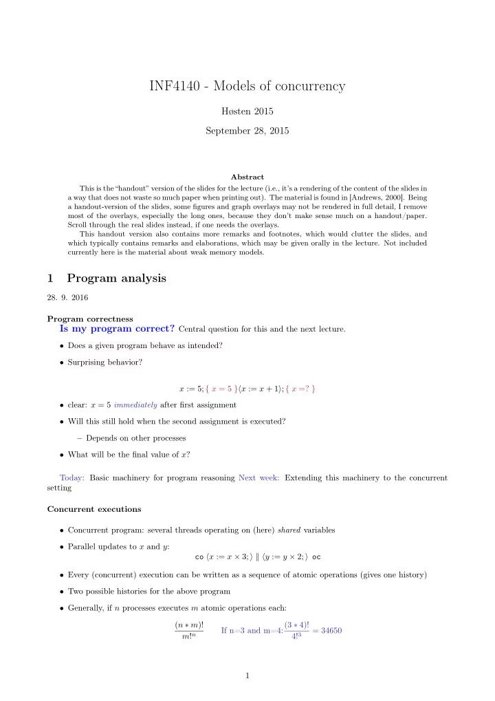
INF4140 - Models of concurrency Høsten 2015 September 28, 2015 Abstract This is the “handout” version of the slides for the lecture (i.e., it’s a rendering of the content of the slides in a way that does not waste so much paper when printing out). The material is found in [Andrews, 2000]. Being a handout-version of the slides, some figures and graph overlays may not be rendered in full detail, I remove most of the overlays, especially the long ones, because they don’t make sense much on a handout/paper. Scroll through the real slides instead, if one needs the overlays. This handout version also contains more remarks and footnotes, which would clutter the slides, and which typically contains remarks and elaborations, which may be given orally in the lecture. Not included currently here is the material about weak memory models. 1 Program analysis 28. 9. 2016 Program correctness Is my program correct? Central question for this and the next lecture. • Does a given program behave as intended? • Surprising behavior? x := 5; { x = 5 }� x := x + 1 � ; { x =? } • clear: x = 5 immediately after first assignment • Will this still hold when the second assignment is executed? – Depends on other processes • What will be the final value of x ? Today: Basic machinery for program reasoning Next week: Extending this machinery to the concurrent setting Concurrent executions • Concurrent program: several threads operating on (here) shared variables • Parallel updates to x and y : co � x := x × 3; � � � y := y × 2; � oc • Every (concurrent) execution can be written as a sequence of atomic operations (gives one history) • Two possible histories for the above program • Generally, if n processes executes m atomic operations each: ( n ∗ m )! If n=3 and m=4: (3 ∗ 4)! = 34650 m ! n 4! 3 1
How to verify program properties? • Testing or debugging increases confidence in the program correctness, but does not guarantee correctness – Program testing can be an effective way to show the presence of bugs, but not their absence • Operational reasoning (exhaustive case analysis) tries all possible executions of a program • Formal analysis (assertional reasoning) allows to deduce the correctness of a program without executing it – Specification of program behavior – Formal argument that the specification is correct States • state of a program consists of the values of the program variables at a point in time, example: { x = 2 ∧ y = 3 } • The state space of a program is given by the different values that the declared variables can take • Sequential program: one execution thread operates on its own state space • The state may be changed by assignments (“imperative”) Example 1 . { x = 5 ∧ y = 5 } x := x ∗ 2 ; { x = 10 ∧ y = 5 } y := y ∗ 2 ; { x = 10 ∧ y = 10 } Executions • Given program S as sequence S 1 ; S 2 ; . . . ; S n ; , starting in a state p 0 : where p 1 , p 2 , . . . p n are the different states during execution • Can be documented by: { p 0 } S 1 { p 1 } S 2 { p 2 } . . . { p n − 1 } S n { p n } • p 0 , p n gives an external specification of the program: { p 0 } S { p n } • We often refer to p 0 as the initial state and p n as the final state Example 2 (from previous slide) . { x = 5 ∧ y = 5 } x := x ∗ 2 ; y := y ∗ 2 ; { x = 10 ∧ y = 10 } Assertions Want to express more general properties of programs, like { x = y } x := x ∗ 2 ; y := y ∗ 2 ; { x = y } • If the assertion x = y holds, when the program starts , x = y will also hold when/if the program terminates • Does not talk about specific, concrete values of x and y , but about relations between their values • Assertions characterise sets of states Example 3 . The assertion x = y describes all states where the values of x and y are equal, like { x = − 1 ∧ y = − 1 } , { x = 1 ∧ y = 1 } , . . . 2
Assertions • state assertion P : set of states where P is true: x = y All states where x has the same value as y x ≤ y : All states where the value of x is less or equal to the value of y x = 2 ∧ y = 3 Only one state (if x and y are the only variables) All states true No state false Example 4 . { x = y } x := x ∗ 2 ; { x = 2 ∗ y } y := y ∗ 2 ; { x = y } Assertions may or may not say something correct for the behavior of a program (fragment). In this example, the assertions say something correct. Formal analysis of programs • establish program properties/correctness, using a system for formal reasoning • Help in understanding how a program behaves • Useful for program construction • Look at logics for formal analysis • basis of analysis tools Formal system • Axioms: Defines the meaning of individual program statements • Rules: Derive the meaning of a program from the individual statements in the program Logics and formal systems Our formal system consists of: • syntactic building blocks: – A set of symbols (constants, variables,...) – A set of formulas (meaningful combination of symbols) • derivation machinery – A set of axioms (assumed to be true) – A set of inference rules Inference rule 1 H 1 . . . H n C • H i : assumption / premise , and C : conclusion • intention: conclusion is true if all the assumptions are true • The inference rules specify how to derive additional formulas from axioms and other formulas. 1 axiom = rule with no premises 3
Symbols • variables: x, y, z, ... (which include program variables + “extra” ones) • Relation symbols: ≤ , ≥ , . . . • Function symbols: + , − , . . . , and constants 0 , 1 , 2 , . . . , true , false • Equality (also a relation symbol): = Formulas of first-order logic Meaningful combination of symbols Assume that A and B are formulas, then the following are also formulas: ¬ A means “not A ” A ∨ B means “ A or B ” A ∧ B means “ A and B ” A ⇒ B means “ A implies B ” If x is a variable and A , the following are formulas: 2 ∀ x : A ( x ) means “ A is true for all values of x ” ∃ x : A ( x ) means “there is (at least) one value of x such that A is true” Examples of axioms and rules (no programs involved yet) Typical axioms: • A ∨ ¬ A • A ⇒ A Typical rules: A B A A ⇒ B A And-I Or-I Or-E A ∧ B A ∨ B B Example 5 . x = 5 y = 5 x = 5 And-I Or-I x = 5 ∧ y = 5 x = 5 ∨ y = 5 x ≥ 0 ⇒ y ≥ 0 x ≥ 0 Or-E y ≥ 0 Important terms • Interpretation : describe each formula as either true or false • Proof : derivation tree where all leaf nodes are axioms • Theorems : a “formula” derivable in a given proof system • Soundness (of the logic): If we can prove (“derive”) some formula P (in the logic) then P is actually (semantically) true • Completeness : If a formula P is true, it can be proven 2 A ( x ) to indicate that, here, A (typically) contains x . 4
Program Logic (PL) • PL lets us express and prove properties about programs • Formulas are of the form “Hoare triple” { P 1 } S { P 2 } – S : program statement(s) – P , P 1 , P ′ , Q . . . : assertions over program states (including ¬ , ∧ , ∨ , ∃ , ∀ ) – In above triple P 1 : pre-condition, and P 2 post-condition of S Example 6 . { x = y } x := x ∗ 2 ; y := y ∗ 2 ; { x = y } The proof system PL (Hoare logic) • Express and prove program properties • { P } S { Q } – P, Q may be seen as a specification of the program S – Code analysis by proving the specification (in PL) – No need to execute the code in order to do the analysis – An interpretation maps triples to true or false ∗ { x = 0 } x := x + 1; { x = 1 } should be true ∗ { x = 0 } x := x + 1; { x = 0 } should be false Reasoning about programs • Basic idea: Specify what the program is supposed to do (pre- and post-conditions) • Pre- and post-conditions are given as assertions over the program state • use PL for a mathematical argument that the program satisfies its specification Interpretation: Interpretation (“semantics”) of triples is related to program execution Partial correctness interpretation { P } S { Q } is true/holds: • If the initial state of S satisfies P ( P holds for the initial state of S ) and • if 3 S terminates, • then Q is true in the final state of S Expresses partial correctness (termination of S is assumed) Example 7 . { x = y } x := x ∗ 2 ; y := y ∗ 2 ; { x = y } is true if the initial state satisfies x = y and, in case the execution terminates, then the final state satisfies x = y 3 Thus: if S does not terminate, all bets are off. . . 5
Recommend
More recommend
Explore More Topics
Stay informed with curated content and fresh updates.


