IN5550: Neural Methods in Natural Language Processing Lecture 2 - PowerPoint PPT Presentation

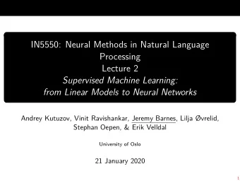
IN5550: Neural Methods in Natural Language Processing Lecture 2 Supervised Machine Learning: from Linear Models to Neural Networks Andrey Kutuzov, Vinit Ravishankar, Lilja Øvrelid, Stephan Oepen, & Erik Velldal University of Oslo 24 January 2019 1

Contents Introduction 1 Basics of supervised machine learning 2 Linear classifiers 3 Training as optimization 4 Limitations of linear models 5 Going deeply non-linear: multi-layered perceptrons 6 Next lecture on January 31 7 Before the next lecture 8 1

Introduction I am Andrey Kutuzov I will do lectures and group sessions in January and February, covering the following topics: ◮ Linear classifiers and simple feed-forward neural networks ◮ Neural language modeling ◮ Dense representations and word embeddings I am also partially responsible for the first 2 obligatory assignments: 1. Bag of Words Document Classification 2. Word Embedding and Semantic Similarity 2

Introduction Technicalities ◮ Make sure to familiarize yourself with the course infrastructure. ◮ Check Piazza and the course page for messages. ◮ Test whether you can access https://github.uio.no/in5550/2019 ◮ make sure to update your UiO github profile with your photo, and star the course repository :-) ◮ Most of machine learning revolves around linear algebra. ◮ We created a LinAlg cheat sheet for this course. ◮ Linked from the course page, adapted for the notation of [Goldberg, 2017] . 3

Contents Introduction 1 Basics of supervised machine learning 2 Linear classifiers 3 Training as optimization 4 Limitations of linear models 5 Going deeply non-linear: multi-layered perceptrons 6 Next lecture on January 31 7 Before the next lecture 8 3

Basics of supervised machine learning ◮ Supervised ML models are trained on example data and produce generalizations. ◮ Supposed to ‘improve with experience’. ◮ Input 1: a training set of n training instances x 1: n = x 1 , x 2 , . . . x n ◮ for example, e-mail messages. ◮ Input 2: corresponding ‘gold’ labels for these instances y 1: n = y 1 , y 2 , . . . y n ◮ for example, whether the message is spam (1) or not (0). ◮ The trained models allow to make label predictions for unseen instances. ◮ Generally: some program for mapping instances to labels. 4

Basics of supervised machine learning Recap on data split ◮ Recall: we want the model to make good predictions for unseen data. ◮ It should not overfit to the seen data. ◮ Thus, the datasets are usually split into: 1. train data; 2. validation/development data (optional); 3. test/held-out data. 5

Basics of supervised machine learning ◮ We want to find a program which makes good predictions for our task. ◮ Searching among all possible programs is unfeasible. ◮ To cope with that, we make ourselves inductively biased... ◮ ...and set some hypothesis class... ◮ ...to search only within this class. A popular hypothesis class: linear functions. 6

Contents Introduction 1 Basics of supervised machine learning 2 Linear classifiers 3 Training as optimization 4 Limitations of linear models 5 Going deeply non-linear: multi-layered perceptrons 6 Next lecture on January 31 7 Before the next lecture 8 6

Linear classifiers Simple linear function f ( x ; W , b ) = x · W + b (1) ◮ Function input: ◮ feature vector x ∈ R d in ; ◮ each training instance is represented with d in features; ◮ for example, some properties of the documents. ◮ Function parameters θ : ◮ matrix W ∈ R d in × d out ◮ d out is the dimensionality of the desired prediction (number of classes) ◮ bias vector b ∈ R d out ◮ bias ‘shifts’ the function output to some direction. 7

Linear classifiers Training of a linear classifier f ( x ; W , b ) = x · W + b θ = W , b ◮ Training is finding the optimal θ . ◮ ‘Optimal’ means ‘ producing predictions ˆ y closest to the gold labels y on our n training instances ’. ◮ Ideally, ˆ y = y 8

Linear classifiers Representing linguistic features ◮ Each of n instances (documents) is represented by a vector of features ( x ∈ R d in ). ◮ Inversely, each feature can be represented by a vector of instances (documents) it appears in ( feature ∈ R n ). ◮ Together these learned representations form a W matrix, part of θ . ◮ Thus, it contains data both about the instances and their features (more about this later). ◮ Feature engineering is deciding what features of the instances we will use during the training. 9

Linear classifiers Here, training instances are represented with 2 features each ( x = [ x 0 , x 1 ]) and labeled with 2 class labels ( y = { black , red } ): ◮ Parameters of f ( x ; W , b ) = x · W + b define the line (or hyperplane) separating the instances. ◮ This decision boundary is actually our learned classifier. ◮ NB: the dataset on the plot is linearly separable. ◮ Question: lines with 3 values of b are shown. Which is the best? 10

Linear classifiers Bag of words ◮ We can have much more features than 2 ◮ (although this is much harder to visualize). ◮ Each word from a pre-defined vocabulary D can be a separate feature. ◮ How many times the word a appears in the document i ? ◮ or a binary flag { 1 , 0 } of whether a appeared in i at all or not. ◮ This schema is called ‘bag of words’ (BoW). ◮ for example, if we have 1000 words in the vocabulary: ◮ i ∈ R 1000 ◮ i = [20 , 16 , 0 , 10 , 0 , . . . , 3] 11

Linear classifiers ◮ Bag-of-Words feature vector of i can be interpreted as a sum of one-hot vectors ( o ) for each token in it: ◮ D extracted from the text above contains 10 words (lowercased): {‘-’, ‘by’, ‘in’, ‘most’, ‘norway’, ‘road’, ‘the’, ‘tourists’, ‘troll’, ‘visited’} . ◮ o 0 = [0 , 0 , 0 , 0 , 0 , 0 , 1 , 0 , 0 , 0] ◮ o 1 = [0 , 0 , 0 , 0 , 0 , 0 , 0 , 0 , 1 , 0] ◮ etc... ◮ i = [1 , 1 , 1 , 1 , 1 , 2 , 2 , 1 , 1 , 1] (‘ the ’ and ‘ road ’ mentioned 2 times) 12

Linear classifiers f ( x ; W , b ) = x · W + b Output of binary classification Binary decision ( d out = 1): ◮ ‘ Is this message spam or not? ’ ◮ W is a vector, b is a scalar. ◮ The prediction ˆ y is also a scalar: either 1 (‘yes’) or − 1 (‘no’). ◮ NB: the model can output any number, but we convert all negatives to − 1 and all positives to 1 ( sign function). θ = ( W ∈ R d in , b ∈ R 1 ) 13

Linear classifiers f ( x ; W , b ) = x · W + b Output of multi-class classification Multi-class decision ( d out = k ) ◮ ‘ Which of k candidates authored this text? ’ ◮ W is a matrix, b is a vector of k components. ◮ The prediction ˆ y is also a one-hot vector of k components. ◮ The component corresponding to the correct author has the value of 1, others are zeros, for example: y = [0 , 0 , 1 , 0] (for k = 4) ˆ θ = ( W ∈ R d in × d out , b ∈ R d out ) 14

Linear classifiers Log-linear classification If we care about how confident is the classifier about each decision: ◮ Map the predictions to the range of [0 , 1]... ◮ ...by a squashing function, for example, sigmoid: 1 y = σ ( f ( x )) = ˆ (2) 1 + e − ( f ( x )) ◮ The result is the probability of the prediction! σ ( x ) 15

Linear classifiers ◮ For multi-class cases, log-linear models produce probabilities for all classes, for example: y = [0 . 4 , 0 . 1 , 0 . 9 , 0 . 5] (for k = 4) ˆ ◮ We choose the one with the highest score: ˆ y = arg max y [ i ] = ˆ ˆ y [2] (3) i ◮ But often it is more convenient to transform scores into a probability distribution, using the softmax function: y = softmax ( xW + b ) ˆ e ( xW + b ) [ i ] (4) y [ i ] = ˆ j e ( xW + b ) [ j ] � ◮ ˆ y = softmax ([0 . 4 , 0 . 1 , 0 . 9 , 0 . 5]) = [0 . 22 , 0 . 16 , 0 . 37 , 0 . 25] ◮ (all scores sum to 1) 16

Contents Introduction 1 Basics of supervised machine learning 2 Linear classifiers 3 Training as optimization 4 Limitations of linear models 5 Going deeply non-linear: multi-layered perceptrons 6 Next lecture on January 31 7 Before the next lecture 8 16

Training as optimization ◮ The goal of the training is to find the optimal values of parameters in θ . ◮ Formally, it means to minimize the loss L ( θ ) on training or development dataset. ◮ Conceptually, loss is a measure of how ‘far away’ the model predictions y are from gold labels y . ˆ ◮ Formally, it can be any function L (ˆ y , y ) returning a scalar value: y ) 2 (square error) ◮ for example, L = ( y − ˆ ◮ It is averaged over all training instances and gives us estimation of the model ‘fitness’. ◮ ˆ θ is the best set of parameters: ˆ θ = arg min L ( θ ) (5) θ 17

Training as optimization Common loss functions 1. Hinge (binary): L (ˆ y , y ) = max (0 , 1 − y · ˆ y ) 2. Hinge (multi-class): L (ˆ y , y ) = max (0 , 1 − (ˆ y [ t ] − ˆ y [ k ] )) 3. Log loss: L (ˆ y , y ) = log (1 + exp ( − (ˆ y [ t ] − ˆ y [ k ] )) 4. Binary cross-entropy (logistic loss): L (ˆ y , y ) = − y log ˆ y − (1 − y ) log (1 − ˆ y ) 5. Categorical cross-entropy (negative log-likelihood): L (ˆ y , y ) = − � y [ i ] log (ˆ y [ i ] ) i 6. Ranking losses, etc, etc... 18