IN5550 Neural Methods in Natural Language Processing Applications - PowerPoint PPT Presentation
IN5550 Neural Methods in Natural Language Processing Applications of Recurrent Neural Networks Stephan Oepen University of Oslo March 24, 2019 Our Roadmap Last Week Language structure: sequences, trees, graphs Recurrent Neural
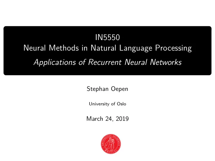
IN5550 Neural Methods in Natural Language Processing Applications of Recurrent Neural Networks Stephan Oepen University of Oslo March 24, 2019
Our Roadmap Last Week ◮ Language structure: sequences, trees, graphs ◮ Recurrent Neural Networks ◮ Different types of sequence labeling ◮ Learning to forget: Gated RNNs Today: First Half ◮ RNNs for structured prediction ◮ A Selection of RNN applications Today: Second Half ◮ Encoder–decoder (sequence-to-sequence) models ◮ Conditioned generation and attention 2
Recap: Recurrent Neural Networks ◮ Recurrent Neural Networks (RNNs) ◮ map input sequence x 1: n to output y 1: n ◮ internal state sequence s 1: n as ‘memory’ RNN ( x 1: n , s 0 ) = y 1: n s i = R ( s i − 1 , x i ) y i = O ( s i ) x i ∈ R d x ; y i ∈ R d y ; s i ∈ R f ( d y ) 3
Recap: The RNN Abstraction Unrolled ◮ Each state s i and output y i depend on the full previous context, e.g. = R ( R ( R ( R ( x 1 , s o ) , x 2 ) , x 3 ) x 4 ) s 4 ◮ Functions R ( · ) and O ( · ) shared across time points; fewer parameters 4
Recap: Bidirectional, Stacked, and Character RNNs 5
Recap: The ‘Simple’ RNN (Elman, 1990) ◮ Want to learn the dependencies between elements of the sequence ◮ nature of the R ( · ) function needs to be determined during training The Elman RNN R ( s i − 1 , x i ) = g ( s i − 1 W s + x i W x + b ) s i = = O ( s i ) = s i y i x i ∈ R d x ; s 1 , y i ∈ R d y ; W x ∈ R d x × d s ; W s ∈ R d s × d s ; b ∈ R d s ◮ Linear transformations of states and inputs; non-linear activation ◮ alternative, equivalent definition of R ( · ) : s i = g ([ s i − 1 ; x i ] W + b ) 6
Recap: RNNs In a Nutshell ◮ State vectors s i reflect the complete history up to time point i ; ◮ RNNs are sensitive to (basic) natural language structure: sequences; ◮ applicable to indeterminate and unlimited length inputs (in principle); ◮ few parameters: matrices W s and W x shared across all time points; ◮ analoguous to (potentially) deep nesting: repeated multiplications; ◮ near-crippling practical limitation: ‘exploding’ or ‘vanishing’ gradients; → gated RNNs: Hochreiter & Schmidhuber (1997) and Cho et al. (2014). 7
Recap: Learning to Forget ⊙ ⊙ ⊙ 8
Recap: Long Short-Term Memory RNNs (LSTMs) ◮ State vectors s i partitioned into context memory and hidden state; ◮ forget gate f how much of the previous memory to keep; ◮ input gate i how much of the proposed update to apply; ◮ output gate o what parts of the updated memory to output. = R( x i , s i − 1 ) = [ c i ; h i ] s i σ ( x i W xf + h i − 1 W hf + b f ) f i = σ ( x i W xi + h i − 1 W hi + b i ) i i = σ ( x i W xo + h i − 1 W ho + b o ) o i = f i ⊙ c i − 1 + i i ⊙ tanh( x i W x + h i − 1 W h + b ) c i = = o i ⊙ tanh( c i ) h i y i = O ( s i ) = h i ◮ More parameters: separate W x · and W h · matrices for each gate. 9
A Variant: Gated Recurrent Units (GRUs) ◮ Same overall goals, but somewhat lower complexity than LSTMs ◮ “substantially fewer gates” (Goldberg, 2017, p. 181): two (one less) = R( x i , s i − 1 ) = (1 − z i ) ⊙ s i − 1 + z i ⊙ ˜ s i s i σ ( x i W xz + s i − 1 W sz + b z ) z i = σ ( x i W xr + s i − 1 W sr + b r ) = r i tanh( x i W x + ( r ⊙ s i − 1 ) W s + b ) s i ˜ = = O ( s i ) = s i y i ◮ Can give results comparable to LSTMs, at reduced training costs: [...] the jury is still out between the GRU, the LSTM, and possible alternative RNN architectures. (Goldberg, 2017, p. 182) 10
Recap: Common Applications of RNNs (in NLP) ◮ Acceptors e.g. (sentence-level) sentiment classification: P ( c = k | w 1: n ) = y [ k ] ˆ softmax(MLP([RNN f ( x 1: n ) [ n ] ; RNN b ( x n :1 ) [1] ])) y ˆ = = E [ w 1 ] , . . . , E [ w n ] x 1: n ◮ transducers e.g. part-of-speech tagging: softmax(MLP([RNN f ( x 1: n ) [ i ] ; RNN b ( x n :1 ) [ i ] ])) [ k ] P ( c i = k | w 1: n ) = x 1: n = E [ w 1 ] , . . . , E [ w n ] ◮ encoder–decoder (sequence-to-sequence) models coming later today 11
Recap: Sequence Labeling in NLP ◮ Token-level class assignments in sequential context, aka tagging ◮ e.g. phoneme sequences, parts of speech; chunks, named entities, etc. ◮ some structure transcending individual tokens can be approximated Michelle Obama visits UiO today . NNP NNP VBZ NNP RB . B PERS I PERS O B ORG O O B PERS E PERS O S ORG O O � 2 , NP � � 1 , S � � 2 , VP � � 2 , VP � � 1 , S � ◮ IOB (aka BIO) labeling scheme—and variants—encodes chunkings. ◮ What is the constituent tree corresponding to the bottom row labels? 12
Two Definitions of ‘Sequence Labeling’ ◮ Hmm, actually, what exactly does one mean by sequence labeling? ◮ gentle definition class predictions for all elements, in context; ◮ pointwise classification; each individual decision is independent; ◮ no (direct) model of wellformedness conditions on class sequence; ◮ strict definition sequence labeling performs structured prediction; ◮ search for ‘globally’ optimal solution, e.g. most probable sequence; ◮ models (properties of) output sequence explicitly, e.g. class bi-grams; ◮ later time points impact earlier choices, i.e. revision of path prefix; ◮ search techniques: dynamic programming, beam search, re-ranking. 13
Wanted: Sequence-Level Output Constraints 14
Recap: Viterbi Decoding—Thanks, Bec! v 2 ( H ) = v 3 ( H ) = max( . 32 ∗ . 12 , . 02 ∗ . 06) max( . 0384 ∗ . 24 , . 032 ∗ . 12) v 1 ( H ) = 0 . 32 = . 0384 = . 0092 v f ( � /S � ) = max( . 0092 ∗ . 2 , P ( H | H ) P (1 | H ) P ( H | H ) P (3 | H ) H H H . 0016 ∗ . 2) P ( H | S ) P (3 | H ) 0 . 6 ∗ 0 . 2 0 . 6 ∗ 0 . 4 P ( C | H ) P (1 | C ) P ( C | H ) P (3 | C ) = . 0018 P ( � /S �| H ) 0 . 8 ∗ 0 . 4 0 . 2 ∗ 0 . 5 0 . 2 ∗ 0 . 1 0 . 2 P ( H | C ) P (1 | H ) P ( H | C ) P (3 | H ) � S � � /S � P ( C | S ) P (3 | C ) 0 . 3 ∗ 0 . 2 ) 0 . 3 ∗ 0 . 4 C | � S 0 . 2 ∗ 0 . 1 / � ( 2 P . 0 P ( C | C ) P (1 | C ) P ( C | C ) P (3 | C ) C C C 0 . 5 ∗ 0 . 5 0 . 5 ∗ 0 . 1 v 1 ( C ) = 0 . 02 v 2 ( C ) = v 3 ( C ) = max( . 32 ∗ . 1 , . 02 ∗ . 25) max( . 0384 ∗ . 02 , . 032 ∗ . 05) = . 032 = . 0016 3 1 3 o 1 o 2 o 3 � � H H H 15
‘Vintage’ Machine Learning to the Rescue Neural Architectures for Named Entity Recognition Guillaume Lample ♠ Miguel Ballesteros ♣♠ Sandeep Subramanian ♠ Kazuya Kawakami ♠ Chris Dyer ♠ ♠ Carnegie Mellon University ♣ NLP Group, Pompeu Fabra University { glample,sandeeps,kkawakam,cdyer } @cs.cmu.edu, miguel.ballesteros@upf.edu Abstract from unannotated corpora offers an alternative strat- egy for obtaining better generalization from small amounts of supervision. However, even systems State-of-the-art named entity recognition sys- tems rely heavily on hand-crafted features and that have relied extensively on unsupervised fea- domain-specific knowledge in order to learn tures (Collobert et al., 2011; Turian et al., 2010; effectively from the small, supervised training Lin and Wu, 2009; Ando and Zhang, 2005b, in- corpora that are available. In this paper, we ter alia ) have used these to augment, rather than introduce two new neural architectures—one replace, hand-engineered features (e.g., knowledge based on bidirectional LSTMs and conditional about capitalization patterns and character classes in random fields, and the other that constructs a particular language) and specialized knowledge re- and labels segments using a transition-based approach inspired by shift-reduce parsers. sources (e.g., gazetteers). Our models rely on two sources of infor- In this paper, we present neural architectures mation about words: character-based word 16
Abstractly: RNN Outputs as ‘Emission Scores’ 17
Conditional Random Fields (CRF) on Top of an RNN ◮ Maybe just maximize sequence probability over softmax outputs? ◮ CRFs mark pinnacle of evolution in probabilistic sequence labeling; ◮ discriminative (like MEMMs), but avoiding the label bias problem; ◮ for an input sequence W = w 1: n and label sequence T = t 1: n e score( W,T ) P ( t 1: n | w 1: n ) = T ′ e score( W,T ′ ) � n +1 n � � score( t 1: n , w 1: n ) = A [ t i − 1 ,t i ] + Y [ i,t i ] i =1 i =1 ◮ Y is the (bi-)RNN ouput; A holds transition scores for tag bi-grams; ◮ What are the dimensionalities of Y and A ? Y ∈ R m × n ; A ∈ R n × n ; ◮ end-to-end training: maximize the log-probability of the correct t 1: n . 18
Some Practical Considerations Variable Length of Input Sequence ◮ Although RNNs in principle well-defined for inputs of variable length, ◮ in practise, padding to fixed length is required for efficiency (batching); ◮ actually not too much ‘waste’; but can be beneficial to bin by length. Evaluation ◮ Accuracy is common metric for tagging; fixed number of predictions; ◮ for most inputs, very large proportion of padding tokens (and labels); ◮ trivial predictions will inflate accuracy scores; detrimental to learning? ◮ Can define custom function: ‘prefix accuracy’; control early stopping? Dropout in RNNs ◮ Dropout along memory updates can inhibt learning of effective gating; ◮ only apply dropout ‘vertically’; or fix random mask (variational RNN). 19
Recommend
More recommend
Explore More Topics
Stay informed with curated content and fresh updates.
