In-operation structural health monitoring: Problems : In-operation - PowerPoint PPT Presentation

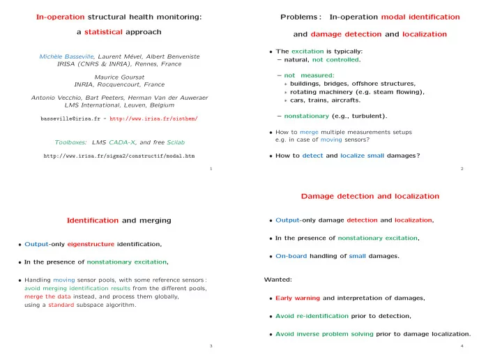
In-operation structural health monitoring: Problems : In-operation modal identification a statistical approach and damage detection and localization • The excitation is typically: Mich` ele Basseville, Laurent M´ evel, Albert Benveniste – natural, not controlled. IRISA (CNRS & INRIA), Rennes, France – not measured: Maurice Goursat ∗ buildings, bridges, offshore structures, INRIA, Rocquencourt, France ∗ rotating machinery (e.g. steam flowing), Antonio Vecchio, Bart Peeters, Herman Van der Auweraer ∗ cars, trains, aircrafts. LMS International, Leuven, Belgium – nonstationary (e.g., turbulent). basseville@irisa.fr - http://www.irisa.fr/sisthem/ • How to merge multiple measurements setups e.g. in case of moving sensors? Toolboxes: LMS CADA-X, and free Scilab • How to detect and localize small damages? http://www.irisa.fr/sigma2/constructif/modal.htm 1 2 Damage detection and localization Identification and merging • Output-only damage detection and localization, • In the presence of nonstationary excitation, • Output-only eigenstructure identification, • On-board handling of small damages. • In the presence of nonstationary excitation, Wanted: • Handling moving sensor pools, with some reference sensors : avoid merging identification results from the different pools, merge the data instead, and process them globally, • Early warning and interpretation of damages, using a standard subspace algorithm. • Avoid re-identification prior to detection, • Avoid inverse problem solving prior to damage localization. 3 4

Modelling Contents M ¨ Z ( s ) + C ˙  Z ( s ) + K Z ( s ) = ν ( s )         FE model:  – Modelling     Y ( s ) = L Z ( s )      – Output-only covariance-driven subspace identification ( Mµ 2 + Cµ + K )Ψ µ = 0 , ψ µ = L Ψ µ – Robustness to nonstationary excitation  X k +1 = F X k + V k         State space:  – Damage detection     Y k = HX k      – Damage diagnostics ∆ F Φ λ = λ Φ λ , ϕ λ = H Φ λ – Examples e δµ = λ , ψ µ = ϕ λ � �� � � �� � modes mode shapes 5 6 Output-only covariance-driven subspace identification Implementation  X k +1 = F X k + V k     Y k = H X k   ˆ ˆ ˆ    R 0 R 1 R 2 . . .        ˆ ˆ ˆ   N R 1 R 2 R 3 . . . ∆   ˆ k =1 Y k Y T ˆ   H =   R i = 1 /N , R 0 R 1 R 2 . . . �   k − i     ˆ ˆ ˆ     R 2 R 3 R 4 . . .       R 1 R 2 R 3 . . .     ∆    Y k Y T   � �� �   H = . . ... . R i = E ,   ok when nonstationary !  . . .    . . .   k − i    R 2 R 3 R 4 . . .       � �� �  . . ... .  ok if stationary ! . . .   . . .   H ≈ ˆ ˆ O ˆ C   � G H C ∆ F 2 G � = F G . . .   → (ˆ SVD ( ˆ → ˆ → ( ˆ H, ˆ HF   H ) + truncation − O − F ) − λ, ˆ ϕ λ ) O ∆   = ,   HF 2     � � G ∆ X k Y T   . = E  .  . k    ∆ 1 0  W T ; H = U ∆ W T ˆ O = U ∆ 1 / 2 ˆ = U 0 ∆ 0 1 R i = H F i G = ⇒ H = O C O ↑ p ( H, F ) = O p ( H, F ) F H − → O − → ( H, F ) − → ( λ, ϕ λ ) det( F − λ I ) = 0 , F Φ λ = λ Φ λ , ϕ λ = H Φ λ 7 8

Robustness to nonstationary excitation Structural monitoring : Eigenstructure monitoring R i ≈ H F i ˆ ˆ G Approximate factorization of covariances :  X k +1 = F X k + V k F Φ λ = λ Φ λ           T − 1 ˆ   ˆ (ˆ ∆  F T → F, H → H ; ϕ λ ) → ( λ, ϕ λ )  Consistency : λ, ˆ  Y k = H X k ϕ λ = H Φ λ      Theory and experience show that the combination of:   Λ modes Canonical parameter : θ ∆ =       vec Φ mode shapes   • the key factorization property of the covariances,   Φ   Φ∆   • the averaging operation in their computation,   O p +1 ( θ ) = Observability in modal basis :   .  .  .      Φ∆ p  allows to cancel out nonstationarities in the excitation. 9 10 Damage detection Subspace model/data correlation (1) θ 0 : reference parameter, known (or identified)  ˆ ˆ ˆ  R 0 R 1 R 2 . . .      ˆ ˆ ˆ   R 1 R 2 R 3 . . .    → ˆ → ˆ Fresh data − R i − H =       ˆ ˆ ˆ   R 2 R 3 R 4 . . .         . . ... .  . . .  Y k : N -size sample of new measurements . . .     Φ       Φ∆   Observability   Build a residual ζ significantly non zero when damage   Nominal model : O ( θ 0 ) =   Φ∆ 2     in modal basis      .  .   .   ? ker O T ( θ 0 ) Local approach (small deviations) ker ˆ H T ! H = O C ! = √ H 0 : H 1 : Test θ = θ 0 against θ = θ 0 + δθ/ N 11 12

Subspace model/data correlation (2) Subspace model/data correlation (3) S T O p +1 ( θ 0 ) = 0; S T S = I s , The residual is asymptotically Gaussian ∃ S, say S ( θ 0 )  N ( 0 , Σ( θ 0 )) P θ 0 under      ζ N ( θ 0 ) →   N ( M ( θ 0 ) δθ, √ Σ( θ 0 )) under P θ 0 + δθ/    N S T ( θ 0 ) ˆ H ≈ 0 Check if : M ( θ 0 ) : mean sensitivity (Jacobian) of residual ζ w.r.t. modal changes (On-board) χ 2 -test in the residual Residual for structural damage monitoring N Σ − 1 M ( M T Σ − 1 M ) − 1 M T Σ − 1 ζ N ζ T ≥ h = vec( S T ( θ 0 ) ˆ ζ N ( θ 0 ) ∆ H ) (On-board) modal χ 2 -test N Σ − 1 M i ( M T i Σ − 1 M i ) − 1 M T i Σ − 1 ζ N How to assess the significance of : S T ( θ 0 ) ˆ ζ T ≥ h H ≈ 0 ? ? 13 14 On-board damage diagnostics: projecting changes Jacobian ? Model/data correlation - Generalization clustering . . . . . . .. .. . . . . . . Any estimating function can play the role of a residual . . .. . . . . Warning: . . . . The prediction error is OK for sensor faults, . . . . FE domain NOT for structural damages ! changes modal domain changes 15 16

Damage diagnostics: (local) sensitivity approach Examples    δM • Sports car ζ ∼ N ( M δθ, δθ = I J ( M ⋆ Σ) ,   0 ,K ⋆   0 )   δK  ( M ⋆ 0 , K ⋆ 0 ) : design model • Z24 bridge J ( M⋆ 0) → ( δµ, δψ µ ) 0 ,K⋆ Jacobian : ( δM, δK ) • Reticular structure Reduction: I matching computed/identified modes   • Slat track  M  ≫ dim θ Problem : dim       K Hint: Cluster the vectors ( δµ, δψ µ ) using the χ 2 -metric • Aircraft flutter monitoring 17 18 Z24 bridge Identified first four natural frequencies / Test values (Results with four sensors) • A benchmark of the BRITE/EURAM project SIMCES χ 2 Mode 1 2 3 4 and of the European COST action F3 Undamaged Freq.(Hz) 3.88 5.01 9.80 10.30 8.80 · 10e2 • Response to traffic excitation under the bridge measured over one year in 139 points Damaged (1) Freq.(Hz) 3.87 5.06 9.79 10.32 8.00 · 10e5 • Two damage scenarios (DS1 and DS2): Damaged (2) Freq.(Hz) 3.76 4.93 9.74 10.25 3.96 · 10e6 pier settlements of 20mm and 80mm. 19 20

Aircraft flutter monitoring • Aero-elastic flutter: critical instability phenomenon • Flight flutter testing procedure Evolution of the test values over three months on a log-scale amplitude. Two different sets of sensors (Left and Right). • Objective : on-line in-flight exploitation of test data • On-line flight flutter monitoring problem: monitoring some specific damping coefficient • Using a different computation of the residual ζ , introducing a minimum magnitude of change, and using the CUSUM test Distribution of the test values for each of the nine months. 21 22 Test for ρ c = ρ (1) . c Test for ρ c = ρ (2) < ρ (1) . c c Bottom: − g − n reflects ρ < ρ c . Top: g + n reflects ρ > ρ c . 23 24