Improved Bounds on the Dot Product under Random Projection and - PowerPoint PPT Presentation
Improved Bounds on the Dot Product under Random Projection and Random Sign Projection Ata Kab an School of Computer Science The University of Birmingham Birmingham B15 2TT, UK http://www.cs.bham.ac.uk/ axk KDD 2015, Sydney, 10-13
Improved Bounds on the Dot Product under Random Projection and Random Sign Projection Ata Kab´ an School of Computer Science The University of Birmingham Birmingham B15 2TT, UK http://www.cs.bham.ac.uk/ ∼ axk KDD 2015, Sydney, 10-13 August 2015.
Outline • Introduction & motivation • A Johnson-Lindenstrauss lemma (JLL) for the dot product without union bound • Corollaries & connections with previous results • Numerical validation • Application to bounding generalisation error of compressive linear classifiers • Conclusions and future work
Introduction • Dot product – a key building block in data mining – classification, regression, retrieval, correlation-clustering, etc. • Random projection (RP) – a universal dimensionality reduc- tion method – independent of the data, computationally cheap, has low-distortion guarantees – The Johnson-Lindenstrauss lemma (JLL) for Euclidean distances is optimal, but for dot product the guarantees have been looser; some suggested that obtuse angles may be not preserved.
Background: JLL for Euclidean distance Theorem [Johnson-Lindenstrauss lemma] Let x, y ∈ R d . Let R ∈ M k × d , k < d , be a random projection matrix with entries drawn i.i.d. from a 0-mean subgaussian distribution with parameter σ 2 , and let Rx, Ry ∈ R k be the images of x, y under R . Then, ∀ ǫ ∈ (0 , 1) : � � − kǫ 2 Pr {� Rx − Ry � 2 < (1 − ǫ ) � x − y � 2 kσ 2 } < exp (1) 8 � � − kǫ 2 Pr {� Rx − Ry � 2 > (1 + ǫ ) � x − y � 2 kσ 2 } < exp (2) 8 An elementary constructive proof is in [Dasgupta & Gupta, 2002]. These bounds are known to be optimal [Larsen & Nelson, 2014].
The quick & loose JLL for dot product � R ( x + y ) � 2 − � R ( x − y ) � 2 � • ( Rx ) T Ry = 1 � 4 Now, applying the JLL on both terms separately and applying the union bound yields: � � − kǫ 2 Pr { ( Rx ) T Ry < x T ykσ 2 − ǫkσ 2 · � x � · � y �} < 2 exp 8 � � − kǫ 2 Pr { ( Rx ) T Ry > x T ykσ 2 + ǫkσ 2 · � x � · � y �} < 2 exp 8 � R ( x − y ) � 2 − � Rx � 2 − � Ry � 2 � • Or, ( Rx ) T Ry = 1 � 2 ...then we get factors of 3 in front of exp.
Can we improve the JLL for dot products? The problems: • Technical issue: Union bound. • More fundamental issue: Ratio of std of projected dot prod- uct and original dot product (‘coefficient of variation’) is unbounded [Li et al. 2006]. • Other issue: Some previous proofs were only applicable to acute angles [Shi et al, 2012]; obtuse angles investigated empirically is inevitably based on limited numerical tests.
Results: Improved bounds for dot product Theorem [Dot Product under Random Projection] Let x, y ∈ R d . Let R ∈ M k × d , k < d , be a random projection matrix having 0-mean subgaussian entries with parameter σ 2 , and let i.i.d. Rx, Ry ∈ R k be the images of x, y under R . Then, ∀ ǫ ∈ (0 , 1) : � � − kǫ 2 Pr { ( Rx ) T Ry < x T ykσ 2 − ǫkσ 2 · � x � · � y �} < exp (3) 8 � � − kǫ 2 Pr { ( Rx ) T Ry > x T ykσ 2 + ǫkσ 2 · � x � · � y �} < exp (4) 8 The proof uses elementary techniques. A standard Chernoff bound argument, but exploit the convexity of the exponential function. The union bound is eliminated. (Details in the paper.)
Corollaries (1): Clarifying the role of angle Corollary [Relative distortion bounds] Denote by θ the angle be- tween the vectors x, y ∈ R d . Then we have the following: 1. Relative distortion bound: Assume x T y � = 0 . Then, | x T R T Ry � � � k � 8( kσ 2 ) 2 ǫ 2 cos 2 ( θ ) − kσ 2 | > ǫ Pr (5) < 2 exp − x T y 2. Multiplicative form of relative distortion bound: � � − k 8 ǫ 2 cos 2 ( θ ) Pr { x T R T Ry < x T y (1 − ǫ ) kσ 2 } < exp (6) � − k � 8 ǫ 2 cos 2 ( θ ) Pr { x T R T Ry > x T y (1 + ǫ ) kσ 2 } < exp (7)
Observations from Corollary • Guarantees are the same for both obtuse and acute angles! • Symmetric around orthogonal angles. • Relation to coefficient of variation [Li et al.]: � Var ( x T R T Ry ) � 2 ≥ k (unbounded) (8) x T y Computing this (case of Gaussian R), � Var ( x T R T Ry ) � � � 1 1 = 1 + (9) x T y cos 2 ( θ ) k we see that unbounded coefficient of variation occurs only when x and y are perpendicular. Again, symmetric around orthogonal angles.
Corollaries (2) Corollary [Margin type bounds and random sign projection] De- note by θ the angle between the vectors x, y ∈ R d . Then, 1. Margin bound: Assume x T y � = 0 . Then, • for all ρ s.t. ρ < x T ykσ 2 and ρ > (cos( θ ) − 1) � x � · � y � kσ 2 , � � 2 � − k � ρ Pr { x T R T Ry < ρ } < exp cos( θ ) − (10) � x � · � y � kσ 2 8 • for all ρ s.t. ρ > x T ykσ 2 and ρ < (cos( θ ) + 1) � x � · � y � kσ 2 , � � 2 � − k � ρ Pr { x T R T Ry > ρ } < exp � x � · � y � kσ 2 − cos( θ ) (11) 8
2. Dot product under random sign projection: Assume x T y � = 0 . Then, � � x T R T Ry � − k � 8 cos 2 ( θ ) Pr (12) < 0 < exp x T y These forms of the bound, with ρ > 0 , are useful for instance to bound the margin loss of compressive classifiers. Details to follow shortly. The random sign projection bound was used before to bound the error of compressive classifiers under 0-1 loss [Durrant & Kab´ an, ICML 13] in the case of Gaussian RP; here subgaussian RP is allowed.
Numerical validation We will compute empirical estimates of the following probabili- ties, from 2000 independently drawn instances of the RP. The target dimension varies from 1 to the original dimension d = 300 . • Rejection probability for dot product preservation = Proba- bility that the relative distortion of the dot product after RP falls outside the allowed error tolerance ǫ : (1 − ǫ ) < ( Rx ) T Ry � � (13) 1 − Pr < (1 + ǫ ) x T y • The sign flipping probability: � ( Rx ) T Ry � Pr < 0 (14) x T y
Replicating the results in [Shi et al, ICML’12]. Left : Two acute angles; Right : Two obtuse angles. Preservation of these obtuse angles looks indeed worse... ...but not because they are obtuse (see next slide!).
Now take the angles symmetrical around π/ 2 and observe the opposite behaviour. – this is why the previous result in [Shi et al, ICML’12] has been misleading. Left : Two acute angles; Right : Two obtuse angles.
Numerical validation – full picture Left : Empirical estimates of rejection probability for dot product preservation; Right : Our analytic upper bound. The error tolerance was set to ǫ = 0 . 3 . Darker means higher probability.
The same with ǫ = 0 . 1 . Bound matches the true behaviour: All of these probabilities are symmetric around the angles of π/ 2 and 3 π/ 2 (i.e. orthogonal vectors before RP). Thus, the preservation of the dot product is symmetrically identical for both acute and obtuse angles.
Empirical estimates of sign flipping probability vs. our analytic upper-bound. Darker means higher probability.
An application in machine learning: Margin bound on compressive linear classification Consider the hypothesis class of linear classifiers defined by a unit length parameter vector: H = { x → h ( x ) = w T x : w ∈ R d , � w � 2 = 1 } (15) The parameters w are estimated from a training set of size N : T N = { ( x n , y n ) } N i.i.d ∼ D over X × {− 1 , 1 } , X ⊆ R d . n =1 , where ( x n , y n ) We will work with the margin loss: 0 if ρ ≤ u ℓ ρ ( u ) = (16) 1 − u/ρ if u ∈ [0 , ρ ] if u ≤ 0 1
We are interested in the case when d is large and N not propor- tionately so. Use a RP matrix R ∈ M k × d , k < d , with entries R ij drawn i.i.d. from a subgaussian distribution with parameter 1 /k . Analogous definitions in the reduced k -dimensional space. The hypothesis class: H R = { x → h R ( Rx ) = w T R Rx : w R ∈ R k , � w R � 2 = 1 } (17) where the parameters w R ∈ R k are estimated from T N R = { ( Rx n , y n ) } N n =1 by minimising the empirical margin error: N 1 ˆ � h R = arg min ℓ ρ ( h R ( Rx n ) , y n ) (18) N h R ∈H R n =1 The quantity of our interest is the generalisation error of ˆ h R as a random function of both T N , and R : � � ˆ E ( x,y ) ∼D (19) h R ( Rx ) � = y
Recommend
More recommend
Explore More Topics
Stay informed with curated content and fresh updates.
