Imprecise probability models for inference in exponential families - PowerPoint PPT Presentation
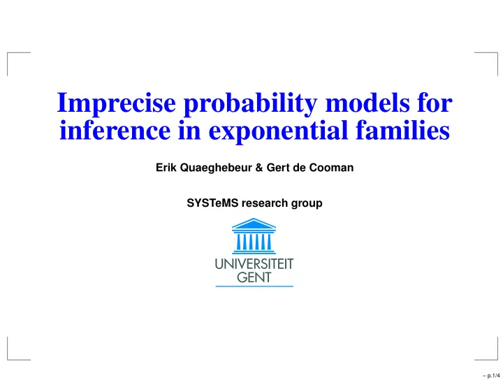
Imprecise probability models for inference in exponential families Erik Quaeghebeur & Gert de Cooman SYSTeMS research group p.1/4 Who we are & what we do Erik Quaeghebeur , PhD student of Gert de Cooman , SYSTeMS research group,
Imprecise probability models for inference in exponential families Erik Quaeghebeur & Gert de Cooman SYSTeMS research group – p.1/4
Who we are & what we do Erik Quaeghebeur , PhD student of Gert de Cooman , SYSTeMS research group, Ghent University, Belgium. – p.2/4
Who we are & what we do Erik Quaeghebeur , PhD student of Gert de Cooman , SYSTeMS research group, Ghent University, Belgium. Current research interests: – p.2/4
Who we are & what we do Erik Quaeghebeur , PhD student of Gert de Cooman , SYSTeMS research group, Ghent University, Belgium. Current research interests: extreme lower probabilities; – p.2/4
Who we are & what we do Erik Quaeghebeur , PhD student of Gert de Cooman , SYSTeMS research group, Ghent University, Belgium. Current research interests: extreme lower probabilities; (partition) exchangeability; – p.2/4
� Who we are & what we do Erik Quaeghebeur , PhD student of Gert de Cooman , SYSTeMS research group, Ghent University, Belgium. Current research interests: extreme lower probabilities; (partition) exchangeability; exponential families. – p.2/4
Socratic dialogue – p.3/4
✁ ✄ ✂ ✂ ✂ ✁ ✁ Our poster: the technical details I Theory on the left. . . E Q & G C SYSTeMS Research Group . . . examples on the right. Department of Electrical Energy, Systems & Automation, Ghent University Technologiepark 914, B-9052 Zwijnaarde, Belgium {Erik.Quaeghebeur,Gert.deCooman}@UGent.be E Let me guide you through. An exponential family Example: Multinomial sampling Consider taking i.i.d. samples x (sample space X ) of a random variable that is dis- In this case, the one sample likelihood function is a multivariate Bernoulli Br ( x | θ ) , the tributed according to an exponential family with probability function of the form conjugate density function is a Dirichlet Di ( θ | ny , ny 0 ) and the predictive mass function is a Dirichlet-multinomial DiMn ( x | ny , ny 0 ) , where Ef ( x | ψ ) = a ( x ) exp( � ψ, τ ( x ) � − b ( ψ )) , � d with functions a : X → R + , b : Ψ → R and with canonical parameter ψ ∈ Ψ and x ∈ { 0 , 1 } d : � x � ≤ 1; θ ∈ (0 , 1) d : � θ � < 1 , θ 0 = 1 − � � ln( θ i i θ i ; τ ( x ) = x ; ψ ( θ ) = θ 0 ) i = 1 ; sufficient statistic τ : X → T . y ∈ (0 , 1) d : � y � < 1 , y 0 = 1 − � Γ ( n ) i y i ; a = 1; b ( ψ ( θ )) = ln( θ 0 ); c ( n , y ) = i Γ ( ny i ) . Γ ( ny 0 ) � The conjugate family Ask me questions. By looking at Ef ( x | · ) as a likelihood function L x : Ψ → R + , we can write down the Example: Normal sampling probability density function of the corresponding family of conjugate distributions, Now, the one sample likelihood function is a Normal N ( x | µ, σ ) , the conjugate density CEf ( ψ | n , y ) = c ( n , y ) exp( n � � ψ, y � − b ( ψ ) � ) , function is a Normal-gamma with normalization factor c and two parameters which can be given specific interpreta- � y 2 − y 12 � n N ( µ | y 1 , n λ ) Ga ( λ | n + 3 tions: a (pseudo)count n ∈ R + and an average sufficient statistic y ∈ Y = co( T ) . , ) 2 2 The predictive family and the predictive density function is a Student St ( x | y 1 , n + 3 1 1 , n + 3) , where n + 1 y 2 − y 2 The probability function of the corresponding family of predictive distributions can be µ ∈ R , λ ∈ R + , σ 2 = 1 derived by by combining L x and CEf ( · | n , y ) , x ∈ R ; λ ; τ ( x ) = ( x , x 2 ); ψ ( λ, µ ) = ( λµ, − 1 2 λ ); � n + 3 � n [ y 2 − y 12 ] 2 c ( n , y ) = 2 √ n � c ( n , y ) a ( x ) y ∈ R × R + : y 2 − y 12 > 0; 1 b ( ψ ( µ, λ )) = λµ 2 − ln( λ ) 2 PEf ( x | n , y ) = CEf ( · | n , y ) L x = . a = √ 2 π ; ; √ . c ( n + 1 , ny + τ ( x ) 2 Γ ( n + 3 2 ) Ψ n + 1 ) 2 π I The conjugate model Example of updating: Multinomial sampling The conjugate model for inference in an exponential family is a lower prevision, defined as the lower envelope of a set of linear previsions that correspond to members of the conjugate family: 2 2 n k − 1 = 2 n k = 3 � P C ( f | n k , Y k ) = inf y ∈Y k P C ( f | n k , y ) , where P C ( f | n k , y ) = CEf ( · | n k , y ) f , f ∈ L ( Ψ ) . “ 1 ” observed Y k − 1 Ψ Y k Here, L ( Ψ ) is the set of all measurable gambles (bounded functions) on Ψ and Y k is 0 1 0 1 some subset of Y . The predictive model Example of updating: Normal sampling The predictive model for inference in an exponential family is defined similarly: � y 2 y 2 P P ( f | n k , Y k ) = inf y ∈Y k P P ( f | n k , y ) , where P P ( f | n k , y ) = PEf ( · | n k , y ) f , f ∈ L ( X ) . X Updating and imprecision A prior choice n 0 and bounded subset Y 0 of Y for the parameters of these models must “ x ” observed be made. When k samples are taken—with sufficient statistic τ k ∈ T —, these can be used to update the models (Bayes’ rule) by obtaining posterior parameters Y k − 1 n 0 y + τ k Y k n k − 1 = 2 n k = 3 n k = n 0 + k , Y k = n 0 + k : y ∈ Y 0 τ ( x ) ⊂ Y . y 1 y 1 The imprecision of the inferences of these models are proportional to the volume of co( Y k ) . So the imprecision decreases with k at a rate that decreases with n 0 . A : Credal classification Example optimization problem: multiple discrete attributes A classifier maps attribute values a ∈ A to one or more classes c ∈ C . In a credal classifier, a conditional lower prevision P ( · | A ) on L ( C ) is used to make pairwise com- parisons of classes c ′ and c ′′ , given attribute values a . The criterion used is c ′ ≻ c ′′ ⇔ inf � � y c ′ y A i | c ′ ∈Y A i | c ′ y a i | c ′ − y c ′′ inf sup y a i | c ′′ . y ∈Y C y A i | c ′′ ∈Y A i | c ′′ c ′ ≻ c ′′ ⇔ P ( I c ′ − I c ′′ | a ) > 0 . i i The inf / sup y A i | c ∈Y A i | c of y a i | c are simple functions of y c that guarantee the convexity of The maximal elements of the resulting strict partial order are the output of the classifier. the objective function. So this problem can easily be solved numerically. The computational complexity of the optimization problem that has to be solved for com- paring two classes c ′ and c ′′ depends highly on the type of attributes that are used. Example optimization problem: one normal attribute The criterion is the same as above, but with the sums replaced by the inf / sup y A| c ∈Y A| c Creating a credal classifier of n A| c + 3 Γ ( n A| c + 4 [ n A| c y A| c , 2 − n A| c y 2 We derive P ( · | A ) by conditioning a joint lower prevision E on L ( C × A ) . E is the � n A| c ) A| c , 1 ] 2 2 . marginal extension of a class model P on L ( C ) and an attribute model P ( · | C ) on L ( A ) . n A| c + 1 Γ ( n A| c + 3 n A| c + 4 ) [ n A| c y A| c , 2 + a 2 − n A| c + 1 [ n A| c y A| c , 1 + a ] 2 ] 1 2 2 When the numer of classes is finite and the attribute values are distributed according to an exponential family, we can use predictive models P P ( · | n C , Y C ) and P P ( · | n A|C , Y A|C ) It is not yet clear if and how this problem can be solved. for the class and attribute models. – p.4/4
Time for questions! ???????????? ? ???? ? ???????? – p.5/4
Recommend
More recommend
Explore More Topics
Stay informed with curated content and fresh updates.
