Impact of Macroprudential Policy Measures on Economic Dynamics: - - PowerPoint PPT Presentation

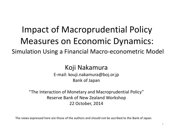
Impact of Macroprudential Policy Measures on Economic Dynamics:

Simulation Using a Financial Macro-econometric Model

Koji Nakamura

E-mail: kouji.nakamura@boj.or.jp Bank of Japan “The Interaction of Monetary and Macroprudential Policy” Reserve Bank of New Zealand Workshop 22 October, 2014

1

The views expressed here are those of the authors and should not be ascribed to the Bank of Japan.

Presentation Outline

• 1. Introduction
• 2. Financial Macro-econometric Model (FMM)
• 3. Simulations and Results
• 4. Discussions and Extensions

2

• 1. Introduction
• Motivation
• Brief Literature Review

3

Motivation

• After the global financial crisis, “financial

cycles” attract more attention of policy makers.

• There is a hope that “macro-prudential

measures” could counter “financial cycles.”

• However, we do not have sufficient

experiences of macro-prudential measures so far.

• We need some “experiments” of macro-

prudential measures to check pros and cons.

4

Brief Literature Review

• Single macro-prudential measure with a small

theoretical model: Cristensen et al. (2011)

• Single macro-prudential measure with a small

empirical model: Aiyar et al. (2012).

• Multiple macro-prudential measures with a

small theoretical model: Angelini et al. (2011) and Goodhart et al (2012).

• Multiple macro-prudential measures with a

large empirical model: This paper.

5

• 2. Financial Macro-econometric Model

(FMM)

• Overview of the FMM
• Structure
• Feedback loop
• Banks’ activities
• “Expectation channel”
• Spending activities
• Monetary policy

6

Overview of the FMM

• The FMM is used for BOJ’s macro stress testing

exercise and is a medium-sized structural model with the detailed financial sector and the macro economic sector.

• About 120 banks* are explicitly modeled with

actual banks’ data such as capital, loan amounts, and transition probabilities.

• The macro economic sector is simpler than other

large scale macro models such as FRB/US, but incorporates a feedback loop between the macro economy and the financial sector.

7

* The latest version of FMM includes 373 banks and has been improved for the financial

• sector. See Kitamura et al. (2014) for the details of the latest version of FMM.

Structure

8

<Financial Sector> Credit cost, Lending interest rate, Capital adequacy ratio, Bank earnings, Lending volume <Macroeconomic Sector> GDP (Corporate capital spending, Household expenditure, etc) Corporate earnings, Employee compensation <Expected Growth and Asset Price Factors> Expected growth rate, Stock prices, Land prices

Model Performance Evaluation

9

Feedback Loop

10

Second-round Effect

11

Banks’ Activities (1)

• Banks’ activities affect the real economy through loan amount

and loan interest rate.

• Bank i’s loan amount to corporate sector

= Bank i’s fixed effect + 1.5*expected growth rate - 1.9*(Bank i’s loan interest rate – CPI ) + 0.4*Bank i’s capital ratio gap + 0.3*land price

• Bank i’s loan interest rate

= Bank i’s fixed effect + 0.95*Bank i’s funding rate + 0.01*loan amount gap

• Bank i’s funding rate

= Bank i’s fixed effect + 0.7*policy rate – 0.1*Bank i’s capital ratio gap

• Land price

= -4.00 + 0.16*nominal GDP growth + 1.03*loan amount (-1) + 1.83*CPI

12

Capital ratio gap is the difference between actual capital ratio and its regulatory level. Loan amount gap is the difference between actual loan amount and its level consistent with potential GDP.

Banks’ Activities (2)

• Individual banks’ credit costs are influenced by the developments of

macro economy and borrowers’ financial condition.

• Bank i’s credit cost

Credit cost = ΣmΣn(transition probability of Bank i’s self-assessment from m to n)* (loss ratio at time of downgrading of Bank i’s self-assessment from m to n)* (exposure of Bank i’s self-assessment of m) Transition probability = Bank i’s fixed effect + α*nominal GDP growth + β*borrowers’ liquid asset-liability ratio*nominal GDP growth + γ*borrowers’ interest coverage ratio*nominal GDP growth

13

The specification of transition probability is revised recently. For more details, see Kitamura et al. (2014).

“Expectation Channel”

• Okina, Shirakawa, and Shiratsuka (2000) : “the intensified

bullish expectations which played an important role behind the large fluctuations in asset prices and the economy.”

• In FMM, real expenditures and asset prices are affected by

expected growth rate.

• Expected growth rate

= 0.77*potential GDP growth rate + 0.10*actual GDP growth rate

• Stock price

= 9.63*corporate profit + 1.39*expected growth rate + 0.32*U.S. stock price

14

Spending Activities

• Household expenditure is affected by expected growth rate

through stock prices and bank loan amount.

• Capital spending by firms is affected by expected growth rate

directly and bank loan amount.

• Household expenditure

= 0.54*labor income + 0.02*stock price + 0.15*loan amount to household – 0.36*loan interest rate

• Capital spending by firms

= 9.0*firm profit + 0.65*expected growth rate – 1.52*(loan interest rate - CPI) + 0.77*loan amount to firms

15

Monetary Policy

• Monetary policy is a simplified Taylor rule.

R(t) = 0.957*R(t-1) + 0.042*output gap(t)

• Since we focus on the average nominal GDP

growth and standard deviation in nominal GDP, price/inflation development is exogenously determined.

• We could extend the model to treat

price/inflation as an endogenous variable.

16

• 3. Simulations and Results
• Simulation procedure
• “Bubble economy shock”
• Macro-prudential measures
• Simulation 1: Fixed duration
• Simulation 2: Various policy strength
• Simulation 3: Recognition lag
• Simulation 4: Use of reference indicators
• Assessment of resilience of financial system

17

Simulation Procedure

• First, we create “the bubble economy” by

producing “shocks” in expected growth rate in

• rder to mimic the actual bubble economy.
• Then, we implement counterfactual

simulations by using the identified “shocks” and macro-prudential policy measures.

• We will look at the average nominal GDP

levels and the standard deviations for both baseline and counterfactual cases.

18

“Bubble Economy”

• As a “baseline” scenario, we create “bubble economy.”
• The expected growth rate is affected by the potential

and actual GDP. If the actual GDP is better than the potential, the optimistic expectations are built.

• Expected growth rate

= 0.77*potential GDP growth rate + 0.1*actual GDP growth rate + shock(t)

• Shock(t)

= iid shock(t) + cumulative growth shock(t)

• Cumulative growth shock(t)

= 0.2*(cumulative growth shock(t-1) + (actual GDP growth rate - potential GDP growth rate) )*I(t), where I(t) = { 1 if the economy is in expansion phase, -1

• therwise}.

19

The parameter of cumulative growth shock (0.2) is set so that the simulation recreates the economic fluctuations during the bubble period in Japan. The duration of I(t) is fixed (4 years) to mimic the actual bubble economy.

Macro-prudential measures

• We use five macro-prudential measures as

follows.

 Time varying capital requirement (countercyclical Capital Buffer, CCB): Regulatory capital adequacy ratio is raised when credit-to-GDP ratio is above a certain threshold.  Credit growth restriction: Restrictions on YoY growth in both household and corporate lending when credit growth is above a certain threshold.  Corporate Loan-To-Value (LTV) regulation: Restrictions on YoY growth in corporate lending when corporate LTV ratio is above a certain threshold.  Retail LTV regulation: Restrictions on YoY growth in household lending when retail LTV ratio is above a certain threshold.  Debt-To-Income (DTI) regulation: Restrictions on YoY growth in household lending when DTI ratio is above a certain threshold.

20

Simulation 1: Fixed duration (1)

• First, we run a simulation in which we use the macro-

prudential measures with fixed duration (1Y, 2Y, 3Y and 4Y).

• For 1Y case, we activate CCB in the first year of the

“bubble” economy, then stop it in the second year. For 2Y, we activate CCB for the first 2 years and stop it in the third year (= the policy duration is 2 years). and so forth…For 4 Y case, we activate CCB for an entire “bubble” period.

• How much should we increase the level of CCB? We

increase the ratio by ¼ σ (=historical standard deviation) as a benchmark case.

• The same “strengths” are used for other macro-prudential

measures: reductions in bank loan amount growth by ¼ σ for the total loan, the household loan, and the corporate loan.

21

Simulation 1: Fixed duration (2)

• The baseline and policy simulations are “visualized” as follows.
• As shown, the baseline scenario shows “big swings.”
• With macro-prudential measures, such “big swings” are repressed, but the

degrees of the policy effects are different.

22 430 440 450 460 470 480 490 1 2 3 4 5 6 7 8 9 10 11 12 13 14 15 Baseline Retail LTV and DTI regulations Corporate LTV regulation Credit growth restrictions Time-varying capital requirement

• tril. yen

years

Simulation 1: Fixed duration (3)

• The vertical line is the difference in the

standard deviations of nominal GDP b/w the baseline and the policy implementation.

• The horizontal line is the difference in

the average nominal GDP b/w the baseline and the policy implementation.

• Trade-off: Both the average and the

standard deviation decline. This is because macro-prudential measures do not push up the economy during the recession period while they do push down the economy during the bubble period.

• Different effects: the effects of various

measures are different. The credit growth restriction is powerful but has a large trade-off. The time-varying capital requirement is less powerful but has a small trade-off.

23

• 7
• 6
• 5
• 4
• 3
• 2
• 1
• 7
• 6
• 5
• 4
• 3
• 2
• 1

Retail LTV and DTI regulations Corporate LTV regulation Credit growth restrictions Time-varying capital requirement nominal GDP, avg., tril. yen

• st. dev., tril. yen

1 year → 2 years → 3 years → 4 years →

Simulation 2: Various policy strength

• Stronger policy measures have

larger impacts. The standard deviations are more reduced when the stronger measures are implemented.

• Trade-offs are more distinct for

stronger policy measures. The stronger policy measures reduce the standard deviations, but at the same time reduce the average nominal GDP.

24

• 12
• 10
• 8
• 6
• 4
• 2
• 12
• 10
• 8
• 6
• 4
• 2

Retail LTV and DTI regulations Corporate LTV regulation Credit growth restrictions Time-varying capital requirement nominal GDP, avg., tril. yen

• st. dev., tril. yen

weaker (1/8σ)→ stronger (1/2σ)→ benchmark (1/4σ)→

Simulation 3: Recognition lag

• The impacts of policy measures

depend on the timing of the policy implementation.

• However, it is difficult to recognize the

state of the economy accurately. Without accurate recognition, the effective policy cannot be

• implemented. This is a typical “real

time issue” for policy implementation.

• The most effective timing of policy

implementation is the third year of the expansion for most policy measures i.e. lower variation and higher average GDP.

• It is harmful to implement measures

after the “bubble economy”. Such actions exacerbate the recession (upper left).

25

• 3
• 2
• 1

1

• 3
• 2
• 1

1 Retail LTV and DTI regulations Corporate LTV regulation Credit growth restrictions Time-varying capital requirement nominal GDP, avg., tril. yen

• st. dev., tril. yen

1st year ↑ ← 2nd year ← 3rd year ← 4th year ← 5th year

Simulation 4: Use of reference indicators

• In a realistic situation, we do not

know when the “bubble economy ” begins and how long the “bubble economy” continues.

• Policy makers need to monitor

“reference indicators” to recognize the state of the economy and decide when they activate the policy measures.

• In the simulations, we assume that

measures are implemented when the reference indicators deviate from their historical trends by 70 or 90 percent confidence intervals.

• The levels of the reference indicators

matter for the impacts of the policy measures.

26

• 5
• 4
• 3
• 2
• 1

1

• 5
• 4
• 3
• 2
• 1

1 Retail LTV regulation Corporate LTV regulation Credit growth restrictions Time-varying capital requirement DTI regulation nominal GDP, avg., tril. yen

• st. dev., tril. yen

90%tile→ 70%tile→

Resilience of Financial System

• Another objective of macro-prudential

policy measures is to build greater resilience of the financial system.

• Average Tier 1 capital ratios under any

policy measures are higher over the financial cycle regardless of which policy measure is implemented.

• Due to higher capital level, loan

amounts during the recession period are higher than those during the baseline case (red circle in RHS chart).

27

(2) Loan amount (1) Tier 1 capital ratio

0.0 0.1 0.2 0.3 0.4

Retail LTV and DTI regulations Corporate LTV regulation Credit growth restrictions Time-varying capital requirement

deviation from the baseline, % pts

• 40
• 30
• 20
• 10

10 1 2 3 4 5 6 7 8 9 10 11 12 13 14 15 Retail LTV and DTI regulations Corporate LTV regulation Credit growth restriction Time-varying capital requirement deviation from the baseline, tril. yen years

• 4. Discussions and Extensions
• Summary of results
• Discussions of the current analysis
• Possible future extensions

28

Summary of Results

• We analyzed the impacts of five macro-prudential

policy measures by using a stress test model (FMM).

• We found the following results.

(1) There are trade-offs between the average economic growth and reduction in the fluctuation of business cycles, depending on macro-prudential measures. (2) Each macro-prudential measures have different impacts on the average economic growth and the fluctuation of business cycles according to the Japanese economic structure. (3) “Real time” issue, the lags between recognition of the state of the economy and implementation of policy measures, is crucial for effectiveness of macro- prudential policy measures. (4) Macro-prudential policy measures can help contribute to more stable financial intermediation by raising the resilience of the financial system against risks.

29

Discussions

• Model

 The model is an econometric model with simple economic structure and not

• DSGE. It is subject to the Lucas critique. Coherent DSGE model would be

preferable, but might be too complicated to be used for policy simulations.

• Policy measures

 We do not know the appropriate size of the policy measures. In monetary policy analysis, the Taylor rule is a benchmark. We do not have such a benchmark among macro prudential policy measures.  We do not know the appropriate combinations of macro prudential policu measures.  The policy impacts are asymmetric. The macro prudential policy measures are used to check the overheating of the economy, but not stimulate the economy in the recession period.

30

Possible Future Extensions

• The combined impacts of monetary policy and

various macro-prudential measures.

• The impacts of macro-prudential measures to

different “shocks”.

• The impacts of liquidity policy measures.
• The appropriate reference indicators.
• Policy simulations with DSGE models.

31

References

Aiyar, S., C. W. Calomiris, and T. Wieladek, 2012, “Does macropru leak? Evidence from a UK policy experiment,” Bank of England Working Paper, No. 445. Angelini, P., S. Neri, and F. Panetta, 2011, “Monetary and macroprudential policies,” Banca d’Italia Working Papers, No. 801. Bank of Japan, Financial System Report. Christensen, I., C. Meh, and K. Moran, 2011, “Bank Leverage Regulation and Macroeconomic Dynamics,” Bank of Canada Working Paper, 2011-32. Goodhart, C. A. E., A. K. Kashyap, D. P. Tsomocos, and A. P. Vardoulakis, 2012, “Financial Regulation in General Equilibrium,” NBER Working Paper Series, 17909. Ishikawa, A., K. Kamada, Y. Kurachi, K. Nasu, and Y. Teranishi, 2012, “Introduction to the Financial Macro-econometric Model,” Bank of Japan Working Paper Series, No. 12-E-1. Kawata, H., Y. Kurachi, K. Nakamura, and Y. Teranishi, 2013, “Impact of Macroprudential Policy Measures on Economic Dynamics: Simulation Using a Financial Macro-econometric Model,” Bank of Japan Working Paper Series, No. 13-E-3. Kitamura, T., S. Kojima, K. Nakamura, K. Takahashi, and I. Takei, 2014, “Macro Stress Testing at the Bank of Japan,” BOJ Reports and Research Papers.

32

Thank you !

33