ImageNet Classification with Deep Convolutional Neural Networks - PowerPoint PPT Presentation

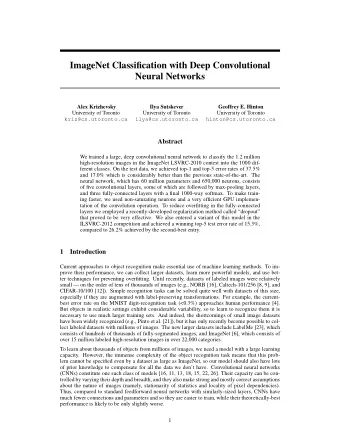
ImageNet Classification with Deep Convolutional Neural Networks Krizhevsky et. all

Outline ● Introduction ● DataSet ● Architecture of the Network ● Reducing overfitting ● Learning Results ● Discussion

Introduction ● A CNN is a neural network with some convolutional layers (and some other layers). ● A convolutional layer has a number of filters that does convolutional operation. ● A neuron is connected to only a spatial region of neurons in the previous layer.

ImageNet ● Over 15M labeled high resolution images. ● Roughly 22K categories. ● Collected from web and labeled by Amazon Mechanical Turk.

ILSVRC ● Annual competition of image classification at large scale. ● 1.2M images in 1K categories. ● Classification: make 5 guesses about the image label.

The Architecture ● Contains eight learned layers ○ Five convolutional ○ Three fully-connected ● Novel or unusual features of the network’s architecture: ○ Relu Nonlinearity ○ Training on multiple GPUs ○ Local Response Normalization ○ Overlapping Pooling

Relu Nonlinearity ● Standard way to model a neuron ○ f(x) = tanh(x) or f(x) = (1 + e -x ) -1 ○ Very slow to train ● Non-saturating nonlinearity (RELU) ○ f(x) = max(0, x) ○ Quick to train

Training on Multiple GPUs ● It turns out that 1.2 million training examples are enough to train networks which are too big to fit on one GPU. ● Therefore the convnet is spread the net across two GPUs. ● The parallelization scheme employed essentially puts half of the kernels on each GPU. ● The GPUs communicate only in certain layers. ● The training took 5 to 6 days on two NVIDIA GTX 580 3GB GPUs. ● This scheme reduces top-1 and top-5 error rates by 1.7% and 1.2%.

Local Response Normalization ● No need to input normalization with ReLUs. ● But still the following local normalization scheme helps generalization. ● Response normalization reduces top-1 and top-5 error rates by 1.4% and 1.2% , respectively.

Overlapping Pooling ● Pooling layer: units spaced s pixels apart, each summarizing a neighborhood of size z × z. ● Traditional Pooling (s=z) ● s < z overlapping pooling ● Top-1 and top-5 error rates decrease by 0.4% and 0.3% respectively with s=2, z=3, compared to the non-overlapping scheme s = 2, z = 2.

Overall Architecture

Convolutional Layer 1 ● Conv layer output: 55*55*96 = 290,400 neurons ● Each has 11*11*3 = 363 weights and 1 bias ● 290400 * 364 = 105,705,600 parameters (on the first layer alone!)

Reduce Overfitting ● 60 million parameters. ● In all, there are roughly 1.2 million training images. ● This turns out to be insufficient to learn so many parameters without considerable overfitting. ● To prevent overfitting: ○ Data Augmentation ○ Dropout

Data Augmentation ● Consists of generating image translations and horizontal reflections. ○ Cropping 224 × 224 patches (and their horizontal reflections) from the 256×256 images. ● The second form of data augmentation consists of altering the intensities of the RGB channels in training images. ● This scheme reduces the top-1 error rate by over 1%.

Dropout ● Simulate having a large number of different network architectures by randomly dropping out nodes during training. ● Dropout offers a very computationally cheap and effective regularization method. ● Probability of 0.5. ● The neurons which are “dropped out” do not contribute to the forward pass and do not participate in backpropagation.

Details of Learning ● Trained the models using stochastic gradient descent. ○ Batch size of 128 examples. ○ Momentum of 0.9, and ○ Weight decay of 0.0005: small amount is important for the model to learn. ● The learning rate is initialized at 0.01 which is adjusted manually throughout training. ○ Divide the learning rate by 10 when the validation error rate stopped improving with the current learning rate.

Results : ILSVRC-2010

Qualitative Evaluations ● 96 convolutional kernels of size 11×11×3 learned by the first convolutional layer on the 224×224×3 input images. ● The top 48 kernels were learned on GPU 1: color-agnostic ● Bottom 48 kernels were learned on GPU 2: color-specific.

ILSVRC-2010 test images

Very Deep Convolutional Networks for Large-Scale Image Recognition Simonyan et. all

The Architecture ● Key Component: very deep ConvNets ○ Upto 19 weight layers ● 3×3 kernels - very small ● Convolutional Stride of 1: ○ No loss of information ● Other Details: ○ Rectification (ReLU) non-linearity ○ 5 max pooling layers ○ 3 Fully Connected Layers

Comparison with AlexNet

Training ● Optimise the multinomial logistic regression objective. ● Mini-batch gradient descent. ○ The batch size was set to 256, momentum to 0.9. The learning rate was initially set to 10 −2 , and then decreased by a factor of 10. ○ ● Fixed-size 224×224 ConvNet input images randomly cropped from rescaled training images. ● Two fixed scales used in training. ○ S = 256 ○ S = 384, used a smaller initial learning rate of 10 −3 . ● Standard Jittering ○ Random horizontal flips ○ Random RGB shifts

Testing ● The fully trained convolutional net is applied to a whole (uncropped) image. ○ The input image is isotropically rescaled to a predefined smallest image side, denoted as Q. ● The result is a class score map with the number of channels equal to the number of classes. ○ The class score map is spatially averaged (sum-pooled) to obtain a fixed-size vector of class scores. ● Augment the test set by horizontal flipping of the images. ● The soft-max class posteriors of original and flipped images are averaged.

Implementation Details ● Implementation is derived from the publicly available C++ Caffe toolbox (Jia, 2013) ● Training and evaluation on multiple GPUs installed in a single system. ○ Train and evaluate on full-size (uncropped) images at multiple scales ● After the GPU batch gradients are computed, they are averaged to obtain the gradient of the full batch. ● Four NVIDIA Titan Black GPUs, training a single net took 2–3 weeks depending on the architecture.

Dataset ● ILSVRC-2012 dataset. ● Includes images of 1000 classes, and is split into three sets: ○ Training (1.3M images) ○ Validation (50K images) ○ Testing (100K images with held-out class labels). ● The classification performance is evaluated using two measures: the top-1 and top-5 error. ● For the majority of experiments, the validation set as the test set.

Single Scale Evaluation

Multi Scale Evaluation

Comparison with the State of the Art

Implementation in Tensorflow

Thank You!