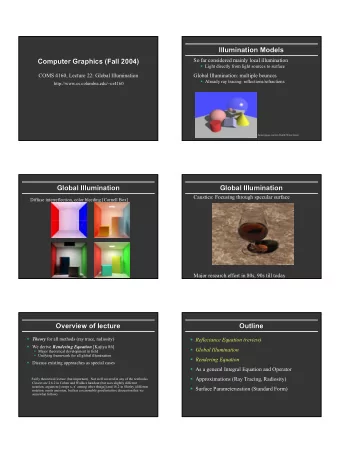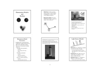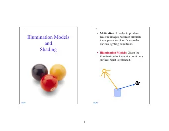
ILLUMINATION MODELS & ALGORITHMS Graphics & Visualization: - PowerPoint PPT Presentation

The Lambert Illumination Model (4) • Let us position dS at a different viewing angle, away from the normal direction of dA, always perpendicular to the corresponding viewing direction vector (see previous figure) • According to Lambert’s cosine law, the new radiance at this arbitrary outbound direction is:     ( cos ) cos d d   0 0 r r L     (12.11) dSd dSd • As dA is very small, the new solid angle dξ’ is proportional to the projection of dA on the light transfer direction ( dξ’ = dAcosθ r /r 2 ), and therefore: d ξ’ = cos θ r d ξ (12.12) 17 Graphics & Visualization: Principles & Algorithms Chapter 12

The Lambert Illumination Model (5) • Replacing the new solid angle in (12.11) yields:      (12.13) cos cos d d d     0 0 0 r r L L      0 cos dSd dSd dSd r • We next derive constant BRDF ( f d ) for the Lambertian surface • Radiant flux is evenly distributed over the hemisphere subtended by the surface patch at vicinity of p , BUT f d is not equal to 1/2 π • Outgoing radiance is constant  does not depend on the reflected light direction on the hemisphere: L r (θ r ,ϕ r ) = L r • Irradiance is not attenuated by the material & is equally spread to every outgoing differential solid angle  reflectance factor     ( ) (ratio of total reflected light to incident light from i d  ) equals 1 i 18 Graphics & Visualization: Principles & Algorithms Chapter 12

The Lambert Illumination Model (6) • From definition of irradiance, radiosity, and radiance ((12.4), (12.5), (12.3)) we get:   (12.14) d E dA i i     ( , ) ( , ) dE dE      r r r r r r ( , ) L    r r r proj cos d d r r r   (12.15)     proj proj dE L d E L d r r r r r r  • Using the results from (12.14) & (12.15), the unit reflectance becomes:     proj proj  dA L d L dA d d r r r r           r ( ) 1  (12.16) i d E dA E dA i i i 19 Graphics & Visualization: Principles & Algorithms Chapter 12

The Lambert Illumination Model (7) • From definition of BRDF & taking into account that BRDF for the Lambertian surface is constant, we have: dL      proj r f dL f L d   d r d i i cos L d i i i        proj proj L f L d f L d f E (12.17) r d i i d i i d i   • Now we can return to (12.16) and substitute L r from (12.17):     proj proj L dA d f E dA d r r d i r      1 E dA E dA i i 1        proj (12.18) f d f f  d r d d  20 Graphics & Visualization: Principles & Algorithms Chapter 12

The Lambert Illumination Model (8) • Summing up:  The radiance associated with an infinitesimal surface patch of area dA around point p is proportional to the cosine of the angle θ i between normal vector at p and the incident direction  The above happens due to the flow of energy that passes through the (projected) area dA of the patch with respect to the incident light direction 21 Graphics & Visualization: Principles & Algorithms Chapter 12

The Phong Illumination Model • The classic local empirical model  Does not take into account the interaction of light between objects • Some of the terms used do not directly derive from physical laws • Gives a reasonable approximation of reality • Modest computational cost  widespread adoption • Proposes a simplified BRDF which:  Relates incoming light intensity from direction (θ i ,φ i ) to reflected light intensity in direction ( θ r ,φ r ) for an object point p   Estimates visible intensity as sum of 4 components:  Emission  Ambient reflection I = I + I + I + I  Diffuse reflection (12.19) e g d s  Specular reflection 22 Graphics & Visualization: Principles & Algorithms Chapter 12

The Phong Illumination Model (2) • Components of the Phong Model: • Emission component I e : caters for objects with self illumination • Ambient component I g : compensates for the fact that the Phong is a local model (thus a surface not directly illuminated by a light source will not appear completely un-illuminated)  ambient light I a : a constant value is assumed  each object reflects ambient light according to its ambient reflectance I g = I a k a (0 ≤ k a ≤ 1) coefficient k a : (12.20) 23 Graphics & Visualization: Principles & Algorithms Chapter 12

The Phong Illumination Model (3) • Light that hits an object directly from a light source is split into 2 reflected components:  Diffusely reflected light, which is uniformly scattered in all directions  Specularly reflected light, which has max value in the “mirror” of the lighting direction • Diffuse & Specular reflection coefficients k d and k s depend mainly on the object’s surface properties  The rougher the surface the more light is diffusely reflected  The shinier the surface the more light is specularly reflected  We have: 0 ≤ kd, ks ≤ 1, kd +ks ≤ 1  Sum of k d and k s may be slightly smaller than 1 to account for light that is transmitted or absorbed by the object  Diffuse component assumes a Lambertian surface & distributes incident light evenly in all directions 24 Graphics & Visualization: Principles & Algorithms Chapter 12

The Phong Illumination Model (4) • Diffuse component does not depend on the viewing direction  Its value is proportional to the irradiance E i which is replaced by intensity I i according to the photometry law (12.8) • The distance d is ignored by assuming the light source at infinity: ˆ          ˆ cos ( · ) , (0 / 2, 0 1) I I k I k n l k d i d i d d where I i the intensity of the point light source, ˆ θ the angle between and ˆ l n  ( k d also depends on the wavelength of the incident light, not modeled here ) 25 Graphics & Visualization: Principles & Algorithms Chapter 12

The Phong Illumination Model (5) ˆ ˆ • Vectors should be unit vectors , l n ˆ ˆ • I d is constant over a planar surface since the vectors are constant , l n ˆ  ˆ • cos θ should be non-negative: max(0, · ) I I k n l d i d • Diffuse component alone gives objects a totally matte appearance • Specular component follows the rule of the mirror ˆ  A perfect mirror will only specularly reflect in the direction of reflection r 26 Graphics & Visualization: Principles & Algorithms Chapter 12

The Phong Illumination Model (6) • Most surfaces have a diminishing function of specular reflection ˆ that attains its max value when the viewing direction coincides v ˆ with : r    ˆ ˆ n n cos ( · ) I I k I k r v (12.22) s i s i s ˆ r ˆ where , are unit vectors & n an empirical value that corresponds v to surface shininess • Specular reflection is responsible for the highlights that are visible on shiny objects • The cos n α term intuitively approximates the spatial distribution of the specularly reflected light 27 Graphics & Visualization: Principles & Algorithms Chapter 12

The Phong Illumination Model (7) • Effect of the material exponent n : • n increases to the right, k s increases upwards: 28 Graphics & Visualization: Principles & Algorithms Chapter 12

The Phong Illumination Model (8) • Small values of n correspond to coarse materials where the size of the highlight is relatively large and scattered • Large values of n correspond to shiny objects with a small and crisp highlight • Specular reflection takes the color of the light source • Example: If a blue object is illuminated by a white light source, the color of the diffuse reflection will be blue but that of the specular reflection will be white • The value of the specular factor cos n α should not take on negative values, so we can replace it by max(0,cos n α) • The Phong model computes the illumination value as: ˆ     ˆ ˆ ˆ n ( ( · ) ( · ) ) (12.23) I I I k I k n l k r v e a a i d s 29 Graphics & Visualization: Principles & Algorithms Chapter 12

The Phong Illumination Model (9) • To simplify computations: Light source & observation point can be ˆ ˆ assumed to be at infinity  constant values for vectors over the , l v area of planar objects • Efficient variant of the specular reflection calculation uses the ˆ ˆ ˆ halfway vector which is the average of : , h l v ˆ  ˆ ( ) / 2 l v ˆ  h (12.24) ˆ  ˆ |( ) / 2| l v 30 Graphics & Visualization: Principles & Algorithms Chapter 12

The Phong Illumination Model (10)         • Angle , angle , and since θ = 2 ϕ +α, we deduce that nh rv  2 rv nh ˆ ˆ ˆ ˆ · • We can thus replace by , and adjust n: · r v nh ˆ ˆ     ˆ ˆ n (12.25) ( ( · ) ( · ) ) I I I k I k nl k nh e a a i d s ˆ ˆ • The vector is much cheaper to compute than r h ˆ ˆ ˆ • If are constant then is also constant h , l v ˆ • can be thought of as the normal vector to the plane for which the h ˆ observer at would see the max value of the specular reflection v ˆ from the light source at l • Since we assumed the light source at infinity, the contribution of the specular and diffuse terms depends on the intensity of the light source and the ambient term is constant 31 Graphics & Visualization: Principles & Algorithms Chapter 12

The Phong Illumination Model (11) • Objects with same properties & orientation but different distances from light will, wrongly, have the same intensity of illumination • Can be corrected by including a factor dependent on the distance of the object point from the light source  Distance factor (physically correct square term often ignored for efficiency):    2 ( ) 1/ ( ) f d c c d c d 1 2 3 • The model thus becomes ˆ ˆ     ˆ ˆ n ( ) ( ( · ) ( · ) ) I I I k f d I k n l k nh e a a i d s • Multiple point light sources can also be handled:  ˆ ˆ     ˆ ˆ n ( ( ) ( ( · ) ( · ) ) ) n l nh I I I k f d I k k , e a a i j d j s j j • For monochromatic light, the original gray level value v of an object point p is thus modified by the result I of the intensity computation: v’ = v I 32 Graphics & Visualization: Principles & Algorithms Chapter 12

The Phong Illumination Model (12) • Color can be handled by giving the color of the light source to the specular reflection • The color of the ambient & diffuse components depends on the color coefficients of the object material • 3 intensity values, one for each of the 3 primary colors, are then computed: ˆ ˆ     ˆ ˆ n ( ( ) ( ( · ) ( · ) )) I I I k f d I k n l k nh r er a ar i dr s ˆ ˆ     ˆ ˆ n (12.28) ( ( ) ( ( · ) ( · ) )) n l nh I I I k f d I k k g eg a ag i dg s ˆ ˆ     ˆ ˆ n ( ( ) ( ( · ) ( · ) )) I I I k f d I k n l k nh b eb a ab i db s • Specular reflection contributes equally to the 3 equations, simulating a white light source  If ( r , g , b ) is the original color of an object at point p , this is modified by the result of the color intensity computation as: ( r' , g' , b' )=( r I r , g I g , b I b ) 33 Graphics & Visualization: Principles & Algorithms Chapter 12

Numerical Example • Let us assume that we want to estimate the intensity value for a point p which, for ease of calculations, lies at the origin of the coordinate system p =[0,0,0] T . Let the normal to the object at p , the light and the viewing vectors respectively be:    T T T [0,2,0] , [1,1,0] , [0, 1, 1] n l v • Suppose the values of the emitted, ambient and incident intensity from the light source are: I e = 2 , I a = 1, I i = 12 • and that the constant values are: k a = 0.3, k d = 0.3, k s = 0.6 and n = 3 34 Graphics & Visualization: Principles & Algorithms Chapter 12

Numerical Example (2) • Light source is twelve times more intense than the ambient light and the object is self-illuminated and emits twice the ambient intensity • k d + k s = 0.9  10% of the incident light is absorbed by the object • Before applying the Phong formula we must compute the halfway vector and normalize all the vectors involved: T T [1,1,0] 1 1 [0,1,1] 1 1 l v ˆ       ˆ T T [ , ,0] , [0, , ] l v   | | | | 2 2 2 2 v 2 2 2 2 l 1 1 1 1 1 1 1 T [ , , ] 1 1 1 1 2 1 h 2 2 2 2 2 ˆ ˆ       ˆ T T ( ) / 2 [ , , ] , [ , , ] , h l v h | | 2 2 2 2 2 3 / 2 2 3 3 2 3 h T [0,2,0]   ˆ T [0,1,0] n 2 2 35 Graphics & Visualization: Principles & Algorithms Chapter 12

Numerical Example (3) • We can now apply equation (12.25): 1 2 I      3 2 1 ·0.3 12·(0.3·( ) 0.6·( ) ) 8.76 2 3  Final intensity value corresponds to the specified viewing angle and is related to the input intensities  The angle between the directions of reflection and viewing is: 2     2 2 ( ) 70 rv nh arccos 3  If the viewing direction coincided with the direction of reflection (i.e. 1 1   ˆ T [ , ,0] ) then the specular reflection would attain its max value v 2 2     since 2 2 (1) : 0 rv nh arccos 1 ˆ       3 T [0,1,0] , 2 1 ·0.3 12·(0.3·( ) 0.6·1 ) 12. 0 5 h I 2 36 Graphics & Visualization: Principles & Algorithms Chapter 12

Phong Model Vectors • The Phong model requires a number of vectors for the computation of the illumination value at a surface point, namely: n, l, v and r or h • Important to use efficient formulae for the computation of these vectors, since such computation is repeated for every point where the model is applied 37 Graphics & Visualization: Principles & Algorithms Chapter 12

The Normal Vector • Defined as a vector perpendicular to a surface at a certain point • Direction of normal vector defines the orientation of the surface • Very useful in computer graphics Normal vector for implicit surfaces: • Implicit surfaces are defined by an equation of the form: f (x, y, z) = 0 • The normal vector at a point p = [ a , b , c ] T of such a surface is given by the gradient vector in the vicinity of p :     / f x      / n f y        /  f z 38 Graphics & Visualization: Principles & Algorithms Chapter 12

The Normal Vector (2) • In the case of a planar surface defined by: f (x, y, z) = ax+by+cz+d = 0 • The normal vector, which is constant over the entire planar surface,  is: [ , , ] T n a b c Normal vector for parametric surfaces: • Surfaces are often represented parametrically • In 3D, a surface is represented by 3 parametric equations in terms of 2 parameters u and v:  ( , ) x f u v x  ( , ) y f u v y  ( , ) z f u v z 39 Graphics & Visualization: Principles & Algorithms Chapter 12

The Normal Vector (3) • The normal vector is then:   f f   n (12.29)   u v where           / / f f u f v x  x  x       f f        , / , / f f f u f v         y y y u v              /   /  f f u f v z z z Normal vector for polygons: • Polygons are the usual building element for model composition • In practice the equation of a polygon’s plane is not known and the polygon is given in terms of a list of its vertices 40 Graphics & Visualization: Principles & Algorithms Chapter 12

The Normal Vector (4) • Given 3 consecutive, non-collinear vertices of a polygon v i− 1 , v i , and v i+1 , we can compute the normal vector:     ( ) ( ) n v v v v i+1 i i-1 i • Cross product is not associative • The above computation follows the right-hand rule: 41 Graphics & Visualization: Principles & Algorithms Chapter 12

The Normal Vector (5) • Must select correct orientation, otherwise normal computations will be reversed & objects will take an “inside - out” look • For polygons with more than 3 vertices, a slight non-planarity may exist  We may compute the polygon normal as the average of the normal vectors given by each pair of consecutive polygon edges  Another technique, due to Martin-Newell: if [ x i , y i , z i ] T , i =1,2, ...,n are the n vertices of a polygon, then the coefficients a,b,c of an approximating plane are computed as: n n n             ( )( ), ( )( ), ( )( ) a y y z z b z z x x c x x y y       1 1 1 1 1 1 i i i i i i i i i i i i    1 1 1 i i i where ⊕ represents addition modulo n The d (constant) coefficient of the plane equation can be computed using the coordinates of a polygon vertex:     ( ) d ax by cz 1 1 1 42 Graphics & Visualization: Principles & Algorithms Chapter 12

The Normal Vector (6) • Another way of computing the normal vector of a polygon: if [ x 1 , y 1 , z 1 ] T , [ x 2 , y 2 , z 2 ] T , and [ x 3 , y 3 , z 3 ] T are 3 non-collinear points, then they must satisfy the plane equation:     1 ax by cz 1 1 1     1 ax by cz 2 2 2     1 ax by cz 3 3 3 • Or        1 1 1 1 x y z a         2 2 2 1 x y z b               3 3 3     1  x y z c • Or XC = D • So C = X −1 D 43 Graphics & Visualization: Principles & Algorithms Chapter 12

Numerical Example • Given polygon with vertices v 1 = [0,0,0] T , v 2 = [1,0,0] T , v 3 = [1,1,0] T , and v 4 = [0,1,0.5] T (slightly non-planar). Compute its normal vector • We shall consider two suitable methods:  1) Average of the normals for each pair of successive edges  2) Martin- Newell’s technique 44 Graphics & Visualization: Principles & Algorithms Chapter 12

Numerical Example (2) Method 1: • We first compute 4 normal vectors • Normals are indexed by the vertex onto which both edges are incident     T T T [1,0,0] [0,1,0.5] [0, 0.5,1] n v 1     T T T [0,1,0] [ 1,0,0] [0,0,1] n v 2      T T T [ 1,0,0.5] [0, 1,0] [0.5,0,1] n v 3        T T T [0, 1, 0.5] [1,0, 0.5] [0.25, 0.5,1] n v 4 • Next, compute the polygon normal by averaging the above • Normalize vectors before summation  give equal weight to all    edges: ˆ ˆ ˆ ˆ n n n n    v v v v T [0.17, 0.22,0.91] , n 1 2 3 4 4   ˆ T [0.18, 0.23,0.96 ] n 45 Graphics & Visualization: Principles & Algorithms Chapter 12

Numerical Example (3) Method 2: • Using Martin- Newell’s technique ,we get:       0·0 ( 1)·0 0·0.5 1 ·0.5 0.5 a        0·1 0·2 ( 0.5)·1 0.5·0 0.5 b       ( 1)·0 0·1 1 ·2 0·0.5 2 c • Thus:   T [0.5, 0.5,2] , n   ˆ T [0.24, 0.24,0.94] n 46 Graphics & Visualization: Principles & Algorithms Chapter 12

Vertex Normal Vector for Polygonal Meshes • Polygonal meshes are often used to approximate objects with smooth change of their surface normal vector • Assume objects that consist of a single manifold surface • In illumination, we need the normal vector to an object’s surface at a discrete set of points covered by the surface :  Determine the normal at the vertices of the polygonal mesh as a weighted average of the normals to the adjacent faces to the vertex  Use this normal to perform bilinear interpolation along edges and finally across edges, on points of the underlying grid • The polygons adjacent to a vertex are the 1-ring neighbors or the star of the vertex 47 Graphics & Visualization: Principles & Algorithms Chapter 12

Vertex Normal Vector for Polygonal Meshes (2) • Vertex normal refers to a weighted average of the normals to the faces of the vertex’s star ˆ • 3 common approaches for computing the unit vertex normal n Approach 1: • Weights can be taken to be equal • Achieved by normalizing the normals of the faces of the star f i before averaging : m   ˆ f i ˆ  1 i n (12.31) m  ˆ | | f i  1 i ˆ  where / | | f f f i i i m : number of faces in the star 48 Graphics & Visualization: Principles & Algorithms Chapter 12

Vertex Normal Vector for Polygonal Meshes (3) Approach 2: • This approach observes that larger polygons should contribute more than smaller ones  Face normals are thus weighted by the area of the corresponding polygons • For triangular faces, this amounts to taking the face normals as computed by the outer product of the vectors represented by 2 of the triangle’s edges  This is because the outer product is equal to twice the area of the triangle m   f i ˆ  1 i n (12.32) m  | | f i  1 i 49 Graphics & Visualization: Principles & Algorithms Chapter 12

Vertex Normal Vector for Polygonal Meshes (4) Approach 3: • This approach observes that in order to ensure that vertex normals are invariant to mesh restructuring, a good weight is the incident angle θ of the faces of the star • Angle θ can be computed by taking the arccos of the dot product of the vectors defined by the incident edges that form it: m   ˆ  f (12.33) i i  ˆ 1 i n m  ˆ  | | f i i  1 i • Note: Vertex normals should be computed before the perspective division (projection) 50 Graphics & Visualization: Principles & Algorithms Chapter 12

Vertex Normal: Symbolic Example • In the following figure m is 6 as there are 6 polygons in the star • In order to evaluate all the vertex normal expressions above, we need ˆ  to compute the , , i f f i i • Take the first triangle v 0 v 1 v 2 : f ˆ    1 , f v v v v f 1 0 1 0 2 1 | | f 1 v v v v   arccos( 0 1 · 0 2 ) 1 | | | | v v v v 0 1 0 2 • Similar computations are performed for the other five triangles in the star and expressions (12.31) – (12.33) can then be evaluated 51 Graphics & Visualization: Principles & Algorithms Chapter 12

Reflection Vector • Reflection vector is computed by noticing that: r ˆ ˆ ˆ  Angles between pairs of vectors ( , ) , ( , ) are equal l n n r ˆ ˆ , , l n r  are coplanar 52 Graphics & Visualization: Principles & Algorithms Chapter 12

Reflection Vector (2) ˆ ˆ • Let be the vector defined by the projection of onto the axis of : r n l 1 ˆ ˆ ˆ ˆ     ˆ ˆ | | | | cos | | ( · ) · , r l l n l n l 1 ˆ since is a unit vector, so: l ˆ   ˆ ˆ ˆ | | ( · ) r n r n n l 1 1 We also have: ˆ     r r t t r l 1 1 • Thus: ˆ ˆ ˆ     ˆ ˆ 2 2 ( · ) r r l n n l l 1 • 6 multiplications and 5 additions are required • When performance is an issue, the reflection vector is replaced by the halfway vector 53 Graphics & Visualization: Principles & Algorithms Chapter 12

Light, View & Halfway Vectors • Light and View vectors are: , l v  either given constant vectors, if the light & view points are placed at infinity,  or simply computed as:   (12.35) l l p   (12.36) v v p where p : object point l : light point v : view point • Halfway vector , useful for specular reflection, is then computed as: h ˆ   (12.37) ˆ ( )/ 2 h l v 54 Graphics & Visualization: Principles & Algorithms Chapter 12

Illumination Algorithms History • Illumination is applied to produce realistic synthetic images • Warnock (1969):  intensity diminishes according to depth  objects were illuminated according to their distance from the light source • Gouraud (1971):  interpolation of intensity values within polygons from intensity values computed at the vertices • Phong :  compute intensity values at every pixel by linearly interpolating vertex normals  using the model he introduced in 1975  there are instances where the linear interpolation of the vertex normals does not work well • Overveld (1997) :  proposed a quadratic interpolation scheme 55 Graphics & Visualization: Principles & Algorithms Chapter 12

Illumination Algorithms based on the Phong Model • Constant shading • Gouraud shading • Phong shading 56 Graphics & Visualization: Principles & Algorithms Chapter 4

Constant Shading • Is the simplest algorithm for polygonal objects • Applies a constant illumination value to each polygonal facet • Incorporated:  Constant ambient lighting  Diffuse reflection • No Specular reflection • The light & view points:  l v  Are both placed at infinity and coincide,  Eliminates shadows ˆ ˆ ( · )  is constant for each polygon n l 57 Graphics & Visualization: Principles & Algorithms Chapter 12

Constant Shading (2) • If the light & view points are on the + z -axis: ˆ   ˆ [0,0,1] T l v  ˆ   ˆ ˆ T  ( · ) for [ , , ] n l n n n n n z x y z • Illumination equation:    I I I k I k n e a a i d z • I is computed once for each polygon  used for all pixels that the polygon covers • Problem:  A polygon mesh often samples a curved surface  The human eye is sensitive to intensity discontinuities  Polygon silhouettes stand out  objects have a “polygonal look” • One solution:  Use some form of illumination interpolation 58 Graphics & Visualization: Principles & Algorithms Chapter 12

Gouraud Shading • Is a simple illumination interpolation algorithm • If the sampling density is sufficiently high, it can capture local maxima (highlights) and minima of shading distribution over the polygon mesh • It computes intensity values for pixels inside a polygon: i. Interpolate the intensity values at its vertices Intensity values at vertices estimated using the Phong model  Use vertex normals to evaluate the Phong equation at the vertices  ii. Bi-linearly interpolate the vertex intensities along the polygon edges & between the edges (along the scanlines)  Scalar interpolation 59 Graphics & Visualization: Principles & Algorithms Chapter 12

Gouraud Shading (2) • Intensities I 1 , I 2 , I 3 are computed using the Phong model • I a , I b : using interpolation between ( I 1 , I 2 , I 3 ):   1 y y y y       2 1 s s ( ( ) ( )) I I I I y y I y y    1 2 1 2 2 1 a s s y y y y y y 1 2 1 2 1 2 1     ( ( ) ( )) I I y y I y y  1 3 3 1 b s s y y 1 3 1 • I s : using interpolation between I a , I b :     ( ( ) ( )) I I x x I x x  s a b s b s a x x b a 60 Graphics & Visualization: Principles & Algorithms Chapter 12

Gouraud Shading (3) • Intensity values are computed incrementally within a scanline: • If s 1 and s 2 are the indices of 2 pixels on the same scanline, then: 1     ( ( ) ( )) I I x x I x x  s a b s b s a 1 x x 1 1 b a 1     ( ( ) ( )) I I x x I x x  s a b s b s a 2 x x 2 2 b a • Subtracting the above equations:   x x x        s s ( ) ( ) I I I 2 1 I I I I   s s s b a b a 2 1 x x x x b a b a  I I • In the case of neighboring pixels ( Δ x =1):   b a I  s x x b a • Incremental intensity computation:    I I I  s , s , 1 s n n 61 Graphics & Visualization: Principles & Algorithms Chapter 12

Phong Shading • Problems of Gouraud Shading:  The sampling density is rarely sufficient to capture highlights  The shading vectors are not interpolated within the polygon but are used to capture intensities at the vertices only  No elimination of mach-bands:  the linear intensity interpolation leaves second-order intensity discontinuities • The Phong algorithm solves the problems of Gouraud shading by applying the Phong model to each pixel covered by a polygon 62 Graphics & Visualization: Principles & Algorithms Chapter 12

Phong Shading (2) • Phong algorithm computations:  The unit normal vectors: bi-linear interpolation from the unit vertex normals 1     ˆ ˆ ( ( ) ( )) n n y y n y y  1 2 2 1 a s s y y 1 2 1     ˆ ˆ n ( n ( ) n ( )) y y y y  b 1 s 3 3 1 s y y 1 3 1     ˆ ˆ ˆ n ( n ( x x ) n ( x x ))  s a b s b s a x x b a  For neighboring pixels on the same scanline, use incremental computation  n n      b x a x n n n n  s x  x x , , 1 s x n s x n s x b a where     n n n n n   b a y y n  s , s , 1 s  y n y n y s y x x b a     n n n n n    b z a z , , 1 n s z n s z n s z  s z x x b a 63 Graphics & Visualization: Principles & Algorithms Chapter 12

Phong Shading (3) • The Phong algorithm:  Is a significant improvement over Gouraud  Requires considerably more computations  Is implemented on graphics accelerators Constant – Gouraud – Phong shading example: 64 Graphics & Visualization: Principles & Algorithms Chapter 12

Quadratic Interpolation of Vertex Normals • Phong shading algorithm  polygonal mesh sufficiently dense  acceptable quality  large polygons  shading artifacts • The silhouette edge problem:  In e.g. below, normal vectors do not vary at all over the surface  Completely flat illumination appearance  This is at odds with the appearance of the silhouette 65 Graphics & Visualization: Principles & Algorithms Chapter 12

Quadratic Interpolation of Vertex Normals (2) • Vertex normal interpolation essentially aims to reconstruct a surface from discrete samples • Reconstruction cannot add information • Tries to come up with a reconstructed surface consistent with the sampled data:  interpolates the vertex normals  is perpendicular to the face normals • The linear interpolation of vertex normals in Phong shading is not consistent in this sense (previous e.g.) 66 Graphics & Visualization: Principles & Algorithms Chapter 12

Quadratic Interpolation of Vertex Normals (3) • Overveld and Wyvill showed that the quadratic interpolation of normals achieves better results ˆ 0 ˆ 1 • If , : the normal vectors to be interpolated and n n  : the vector defined by the subtraction of the 1 st from the last interpolation point • Then the interpolated vector is: ( ) n s     ˆ 2 ( ) with [0..1] and n s n s a s b s 0    ˆ ˆ ( )· n n     ˆ ˆ 0 1 , 3( ) a n n b b 1 0  2   • As expected: ˆ ˆ (0) and (1) n n n n 0 1 • Implemented by taking the forward differences of the quadratic function, at a cost of 2 vector additions per pixel 67 Graphics & Visualization: Principles & Algorithms Chapter 12

Quadratic Interpolation of Vertex Normals (4) • Linear (left) vs Quadratic (right) vector interpolation: flat quadratic linear linear/dense mesh 68 Graphics & Visualization: Principles & Algorithms Chapter 12

Numerical Example • Given the triangle mesh:    T T T [2,2,1] [6,2,1] [4,5,1] v v v 0 1 2      T T T [ 1, 1,1] [1,0,0] [0,1,1] n n n v v v 0 1 2    T T T [2.66,3,1] [5.33,3,1] [4,3,1] a b s • Assume emitted, ambient & incident intensities from light source: I e = 2, I a = 1, I i = 12 • And constant values: k a = 0.3 , k d = 0.3, k s = 0.6, n = 3 • Also assume the light and view points at infinity on the + z -axis : ˆ   ˆ [0,0,1] T l v 69 Graphics & Visualization: Principles & Algorithms Chapter 12

Numerical Example – Constant Shading • Compute the polygon normal:      T ( ) ( ) [0,0,12] n v v v v 1 0 2 0  ˆ T or [0,0,1] n • From equation I = I e + I a k a + I i k d n z : I     5 9 2 1 · 0.3 12 ·0.3 · 1 . 70 Graphics & Visualization: Principles & Algorithms Chapter 12

Numerical Example – Gouraud Shading • Normalize the vertex normals: 1 1 1 1 1      ˆ ˆ ˆ T T T [ , , ] [1,0,0] [0, , ] n n n v v v 0 3 3 3 1 2 2 2 • Use the Phong model to compute the intensities at the vertices: ˆ ˆ      ˆ ˆ 3 2 1 ·0.3 12(0.3( · ) 0.6( · ) ) 5.76 n l n h I v v v 0 0 0 ˆ ˆ      ˆ ˆ 3 2 1 ·0.3 12(0.3( · ) 0.6( · ) ) 2.3 I n l n h v v v 1 1 1 ˆ ˆ      ˆ ˆ 3 2 1 ·0.3 12(0.3( · ) 0.6( · ) ) 7.39 n l n h I v v v 2 2 2 • From Gouraud shading equation: 1 (1    · 2· ) 6.3 I I I a v v 3 2 0 1 (1    · 2· ) 4.0 I I I b v v 3 2 1 1    (1.33· 1.33· ) . I I I 5 13 s a b 2.67 71 Graphics & Visualization: Principles & Algorithms Chapter 12

Numerical Example – Phong Shading • Compute the normals at the edge points a , b from the unit vertex normals (by linear interpolation): 1     ˆ ˆ T (1· 2· ) [ 0.39,0.15,0.62] n n n a v v 3 2 0 1    ˆ ˆ T (1· 2· ) [0.67,0.71,0.71] n n n b v v 3 2 1 • Convert them to unit vectors:    ˆ ˆ T T [ 0.52,0.2,0.83] , [0.55,0.59,0.59] n n a b • Compute the unit normal vector at scanline point s 1     ˆ ˆ T T (1.33 · 1.33 · ) [0.02,0.4,0.71] [0.02,0.49,0.87] n n n s a b 2.67 ˆ s • Apply the Phong model using the unit normal vector : n ˆ ˆ I      ˆ ˆ 3 2 1 ·0.3 12(0.3( · ) 0.6( · ) ) . n l n h 10 25 s s s 72 Graphics & Visualization: Principles & Algorithms Chapter 12

Numerical Example • Phong shading gives significantly higher intensity value compared to Constant or Gouraud shading • This is explained by the existence of a highlight at s • The quadratic interpolation scheme computes I s similarly to Phong  The only difference is the quadratic formulae used for the computation of ˆ ˆ ˆ , and n n n a b s 73 Graphics & Visualization: Principles & Algorithms Chapter 12

The Cook-Torrance Illumination Model* • Problems with the Phong model:  Objects often appear too plastic  The metallic shine or the off-specular-direction highlights are not captured correctly for many shiny materials  The reflected light scattering distribution due to the geometric variation of a rough surface cannot be captured • Cook – Torrance Model:  Extension of the Phong model  General illumination model for rough surfaces  Takes into account the directional distribution and the wavelength dependence of the reflected light 74 Graphics & Visualization: Principles & Algorithms Chapter 12

The Cook-Torrance Illumination Model (2) • Distinguishes the reflected light into :  The ambient term  The diffuse scattering  T he specular highlight • Provides a modeling & parameterization of the BRDF f r of a material • The BRDF f r is linearly composed of :  a pure diffuse term  a pure specular term     , 1 f k f k f k k r d d s s d s 75 Graphics & Visualization: Principles & Algorithms Chapter 12

The Cook-Torrance Illumination Model (3) • The Cook-Torrance reflectance model for N L light sources: N  L ˆ    d  ˆ ( ) ( ) ( ) l l l ( · ) [ ] I I f I n l k f k f r a a i s s d d i  1 l where: ˆ l ( ) l ( )  : the incident light intensity from light source l located at a direction I l i  ( ) l through a solid angle i ˆ n  : the normal vector at the given surface location • I a f a is the ambient term & I a can be regarded as constant • f d is the diffuse BRDF of a Lambertian surface • f a uses the same distribution as f d • The specular part of the BRDF depends on:  the relative location of the observer  the properties of the material 76 Graphics & Visualization: Principles & Algorithms Chapter 12

The Cook-Torrance Illumination Model (4) • In the original paper I a was multiplied by a visibility factor f :  f is the amount of incoming ambient light that was not blocked by the surrounding environment  A distant uniformly luminous hemisphere radiates light toward the inspected surface point p ˆ ( , ) V p l  Uses a binary visibility function with max value 1 when there is a clear line of sight between point p and the surrounding distant hemisphere in ˆ direction : l  ˆ  ˆ ˆ     ˆ ˆ ( · ) ( · ) ( , ) f n l d n l V p l d  unblocked  77 Graphics & Visualization: Principles & Algorithms Chapter 12

The Cook-Torrance Illumination Model (5) • The micro-facet model of Torrance and Sparrow is used for the derivation of the specular term f s  a surface is assumed to be composed of long symmetric V-shaped grooves  each groove consists of two planar facets • The facets:  Are tilted at equal but opposite angles to the surface normal at dA  Are considered perfect mirrors  Reflect light only in the direction of perfect reflection  The slope of the facets (polar angle) θ a determined by a statistical  The orientation of the cavities (azimuth) φ a distribution for the material 78 Graphics & Visualization: Principles & Algorithms Chapter 12

The Cook-Torrance Illumination Model (6) • da : the area of a micro-facet • dA : the inspected area, where reflectance is calculated • In order for the Torrance-Sparrow model to work:  da << dA  wavelength λ of the incident light << micro-facet dimensions   avoid interference phenomena  be able to work with geometrical optics  dispense with wave theory • Cook-Torrance model depends on  Micro-facet distribution term D  Geometric term G  Fresnel term F 79 Graphics & Visualization: Principles & Algorithms Chapter 12

The Cook-Torrance Illumination Model (7) The Micro-facet distribution D ˆ • Is the fraction of micro-facets aligned with direction h • The contribution of each facet is binary : ˆ ˆ to  light reflected fullyfrom direction l v  or, no light reflected at all • Determines the fraction of incident light reflected back to the environment in the direction of view. Several possibilities: • Gaussian distribution (easier to compute)   2  ( / ) a m · D c e ( ) Gaussian • Beckmann distribution (more physically correct) 1   2  (tan / ) a m · D e  ( ) Beckmann 2 4 cos m a where m : the RMS slope of the surface ˆ ˆ θ a : the angle between the normal of dA and of da n h 80 Graphics & Visualization: Principles & Algorithms Chapter 12

The Cook-Torrance Illumination Model (8) • The larger m is :  the more rough the surface  the specular highlight is spread out • Small m : ˆ n  Micro-facets with normal vectors closer to  The material has a polished look  Specular highlight is tighter 81 Graphics & Visualization: Principles & Algorithms Chapter 12

The Cook-Torrance Illumination Model (9) Incoming light interception • Some of the outgoing light in the direction of is attenuated due to v the interception by blocking geometry • The amount of blocking depends on  the outgoing direction ˆ  the slope of the micro-facet relative to n • The amount of light blocked due to light interception is:  [0,1] G intercept ˆ ˆ ˆ ˆ 2( · )( · ) n h n v  G ˆ intercept ˆ · v h 82 Graphics & Visualization: Principles & Algorithms Chapter 12

The Cook-Torrance Illumination Model (10) Shadow ˆ • Some of the light incoming from a direction on a facet da is l blocked by the opposite facet of the groove • This leaves the lower part of the micro-facet in shadow ˆ ˆ ˆ ˆ ˆ ˆ ˆ ˆ 2( · )( · ) 2( · )( · ) nh n l nh n l   G ˆ ˆ ˆ shadow ˆ · · l h vh Combining, Geometric attenuation factor G ˆ ˆ ˆ ˆ ˆ ˆ ˆ ˆ 2( · )( · ) 2( · )( · ) nh n v nh n l G  min{1, , } ˆ ˆ ˆ ˆ · · v h v h 83 Graphics & Visualization: Principles & Algorithms Chapter 12

The Cook-Torrance Illumination Model (11) • Spectral composition for Cook-Torrance model: 1. Diffuse part of BRDF  Is constant  Equal to the reflectance at normal incidence 2. Specular part of BRDF  Is associated with the angle of incidence  It leads to a color shift when the direction of incidence and reflection are at grazing angles 84 Graphics & Visualization: Principles & Algorithms Chapter 12

The Cook-Torrance Illumination Model (12) The Fresnel term F • Describes how a single micro-facet reflects light • Implements the dependence on:  n : the relative index of refraction of the material  k : the extinction coefficient In the Cook-Torrance model • For k = 0 and unpolarized light, the Fresnel equation is:    2 2 1 ( ) [ ( ) 1] g c c g c   (1 ) F    2 2 2 ( ) [ ( ) 1] g c c g c where ˆ  ˆ · v h c    2 2 1 g n c 85 Graphics & Visualization: Principles & Algorithms Chapter 12

The Cook-Torrance Illumination Model (13) The Fresnel term F • F  1 ˆ  ˆ and tends to / 2  The angle between v h  When we look at the direction of the light source from a very low position with respect to the surface ( grazing angle )  Is independent of the n and k values  At a grazing angle, the spectral composition of the reflected light is the same as that of the light source • F ≠ 1 for other angles • k = 0 is also true for non-metals • The Fresnel equation produces a good approximation for metals 86 Graphics & Visualization: Principles & Algorithms Chapter 12

The Cook-Torrance Illumination Model (14) • The specular part of the BRDF:  Gathering D , G , F in a single equation: 1 DGF  f ˆ  s ˆ ˆ ˆ ( · )( · ) n l n v ˆ ˆ ˆ ˆ  maximizes the specular highlight when viewing the light source from ( · )( · ) n l n v a grazing angle Approximation of Cook and Torrance:  Since the calculation of the Fresnel term is expensive 1. Measure/estimate the reflected color at normal incidence F 0 via the Fresnel equation 87 Graphics & Visualization: Principles & Algorithms Chapter 12

The Cook-Torrance Illumination Model (15)  2. At grazing angle for all wavelengths  ( 1) F  /2  (R, G, B) of the reflected light = (R,G,B) of the incident light  The reflected specular color component at an angle may be interpolated:    max(0, ( ) ( )) F F     0 ( ) c c c c    ,0 ,0 i i i ( ) F F , i  2 0 2 where  c i : the color components ( i =R,G,B ) of the resulting color  c i, π/2 : the color components of the material color at normal incidence  c i,0 : the color components of the incident light color 3. The final color c i is:     1 [ max(0, ( ) ( )) ( ) F F DGF      0 ( ) ] c c c c  ˆ    i i ,0 i ,0 ( ) ˆ ˆ ˆ F F ( · )( · ) n l n v i ,  2 0 2 88 Graphics & Visualization: Principles & Algorithms Chapter 12

The Cook-Torrance Illumination Model (16) 89 Graphics & Visualization: Principles & Algorithms Chapter 12

The Oren-Nayar Illumination Model • So far the diffuse component of illumination was based on the Lambertian principle, i.e. equal brightness from all view directions  Works well for smooth surfaces  Rough surfaces are not in general Lambertian  E.g. Full Moon, clay, cement and sand • A rough surface exhibits phenomena such as  Light masking and shadows  Secondary reflections of light on the walls of the irregular microscopic structures  => Brightness of the reflected light increases as the viewing direction approaches the light direction • Oren and Nayar model: Incorporates the above factors to predict the diffuse behavior of rough materials   Adopts the micro-facet model of Torrance-Sparrow  A rough surface consists of long V-shaped grooves 90 Graphics & Visualization: Principles & Algorithms Chapter 12

The Oren-Nayar Illumination Model (2) • The facets are Lambertian surfaces (not perfect mirrors) ˆ The reflected light in direction ( θ r , φ r ) from incident direction is computed as: l  1 ( L     The 1 st order reflected radiance i. , , , ) r r r i i  The light directly reflected in direction from a micro-facet ˆ v L     2 ( The 2 nd reflected radiance ii. , , , ) r r r i i  The light reflected in the same direction after having bounced off the opposite facet of the groove 91 Graphics & Visualization: Principles & Algorithms Chapter 12

The Oren-Nayar Illumination Model (3) • Projected Radiance the contribution of a facet to the total radiance of patch dA    ( , ) d    r a a ( , ) (12.53) L    rp a a ( cos )cos da d a r r where θ a : the slope of the facet wrt surface tangent plane • From the relation between L, E and Φ :            ˆ ˆ   ( , ) ( , )cos ( , )( · ) dE L d L a v d r r r r r r r r r r r r        ( , ) ( , )  d dE da r r r r r r        ˆ ˆ ( , ) ( , )( · ) a v d L d da r r r r r r r   • Substituting radiant flux in (12.53), becomes ( , ) L rp a a      ˆ ˆ ˆ ˆ ( , )( · ) ( , )( · ) a v a v L d da L     r r r r r r r ( , ) (12.55) L    ˆ ˆ ˆ rp a a ˆ ( cos )cos ( · )( · ) da d an v n a r r 92 Graphics & Visualization: Principles & Algorithms Chapter 12

The Oren-Nayar Illumination Model (4) • Micro-facets are Lambertian  BRDF is constant & equal to 1/ π • From the definition of BRDF:  ˆ ˆ             ˆ ˆ ( , ) ( , ) cos ( · ) ( · ) L f E f E f E l a E l a  r r r d i i i d 0 i d 0 0 where ρ = the surface albedo E 0 = the irradiance from the source at normal incidence • Replacing the radiance in (12.55): ˆ ˆ  ˆ ˆ ( · )( · ) l a a v    ( , ) L E  0 ˆ ˆ ˆ rp a a ˆ ( · )( · ) an v n 93 Graphics & Visualization: Principles & Algorithms Chapter 12

The Oren-Nayar Illumination Model (5) • The contribution of all facets facing in the direction of ˆ : a                 1 /2 2 1 ( , , , ) ( , ) ( , )sin (12.58) L P L d d     0 0 r r r i i a a rp a a a a a a a • Geometric factor is a generalization of the Cook-Torrance factor G ˆ  works for any facet normal a ˆ  not necessarily the halfway vector between the viewing and the incident h direction    ˆ ˆ    ˆ ˆ ˆ ˆ ˆ ˆ  2( · )( · ) 2( · )( · ) l n an v n an     min 1,max 0, , GAF ˆ ˆ ˆ ˆ ·      · v a   l a  • Taking also into account the blocked incident and reflected light, (12.58) becomes:                 1 /2 2 1 ( , , , ) ( , ) ( , ) sin L P L GAF d d     0 0 r r r i i a a rp a a a a a a a 94 Graphics & Visualization: Principles & Algorithms Chapter 12

The Oren-Nayar Illumination Model (6) • Radiance from second-order reflections : 95 Graphics & Visualization: Principles & Algorithms Chapter 12

The Oren-Nayar Illumination Model (7)   • The overall radiance leaving patch dA in the direction : ˆ ( , ) v r r               1 2 ( , , , ) ( , , , ) ( , , , ) (12.61) L L L r r r i i r r r i i r r r i i • Simplification of the original model:                     1 ( , , , ) cos [ cos( ) tan (1 | cos( ) |) tan( )] L E C C C  0 1 2 3 r r r i i i r i r i 2    2 2           2 2 ( , , , ) 0.17 cos [1 ( ) cos( )] L E  0    r r r i i i r i 2 0.13 where  2   1 0.5 C   1 2 0.3   2      0.45 sin , cos( ) 0     2 r i 0.09   C 2   2  2   3 0.45 (sin ( ) ), otherwise      2 0.0 9   2 4  2 0.125 ( ) C    3 2 2 0.09         max( , ), min( , ) r i r i 96 Graphics & Visualization: Principles & Algorithms Chapter 12

The Oren-Nayar Illumination Model (8) • The BRDF is acquired by applying the BRDF definition to (12.61):         ( , , , ) ( , , , ) L L    r r i i r r i i f   Oren Nayar cos E E 0 i i          1 2 ( , , , ) ( , , , ) L L r r r i i r r r i i  cos E 0 i 97 Graphics & Visualization: Principles & Algorithms Chapter 12

The Strauss Illumination Model • Illumination models based on geometrical optics (Blinn, Cook- Torrance and Oren-Nayar)  Produce very realistic shading  But, use actual physical parameters found in material science which are generally unintuitive for users (e.g. artists) • The Phong model  Cannot effectively capture the appearance of metallic surfaces  The specular exponent is specified as an unbounded positive number   Cannot easily produce a balanced shininess between a dull surface & a fully reflective one by adjusting its value between two limits  The shininess adjustment is complex  Two seemingly independent parameters (the exponent and the specular coefficient) control the same material attribute 98 Graphics & Visualization: Principles & Algorithms Chapter 12

The Strauss Illumination Model (2) • Strauss Illumination Model:  Borrows many lighting calculations from Phong  Incorporates features like  metallic appearance  off-specular reflections  unified shininess control through intuitive normalized parameters  Empirical model (targeting animators and 3D modelers) • Normalized parameters that control surface appearance: i. The material color c = ( r , g , b ) : represents the albedo of the surface The smoothness s : – ranges from 0 (dull surface) to 1 (perfect mirror) ii. – controls : the specular/diffuse contribution ratio the size of the highlight The metalness m : – is ranges from 0 to 1 (metallic surface) i. – affects the color of the specularly reflected light 99 Graphics & Visualization: Principles & Algorithms Chapter 12

The Strauss Illumination Model (3) • The intensity of the reflected light per color channel c r :    ( ) c c Q Q Q r i d s a where  c i : the corresponding incident light component  Q d , Q s , Q a : the diffuse, specular and ambient components of the Strauss model • The amount of diffuse illumination Q d :  Depends on the shininess of the surface s  The more shiny the surface, the less it behaves as a Lambertian reflector  Decreases with the increase of the metalness m  Depends on the angle of incidence 100 Graphics & Visualization: Principles & Algorithms Chapter 12