I ntroduction to Mobile Robotics Bayes Filter Extended Kalm an - PowerPoint PPT Presentation
I ntroduction to Mobile Robotics Bayes Filter Extended Kalm an Filter Wolfram Burgard 1 Bayes Filter Rem inder Prediction Correction Discrete Kalm an Filter Estimates the state x of a discrete-time controlled process with a
I ntroduction to Mobile Robotics Bayes Filter – Extended Kalm an Filter Wolfram Burgard 1
Bayes Filter Rem inder Prediction Correction
Discrete Kalm an Filter Estimates the state x of a discrete-time controlled process with a measurement 3
Com ponents of a Kalm an Filter Matrix (nxn) that describes how the state evolves from t -1 to t without controls or noise. Matrix (nxl) that describes how the control u t changes the state from t -1 to t. Matrix (kxn) that describes how to map the state x t to an observation z t . Random variables representing the process and measurement noise that are assumed to be independent and normally distributed with covariance Q t and R t respectively. 4
Kalm an Filter Update Exam ple prediction measurement correction It's a weighted mean! 5
Kalm an Filter Update Exam ple prediction correction measurement
Kalm an Filter Algorithm Algorithm Kalm an_ filter ( µ t-1 , Σ t-1 , u t , z t ): 1. 2. Prediction: 3. 4. 5. Correction: 6. 7. 8. Return µ t , Σ t 9.
Nonlinear Dynam ic System s Most realistic robotic problems involve nonlinear functions
Linearity Assum ption Revisited
Non-Linear Function Non-Gaussian!
Non-Gaussian Distributions The non-linear functions lead to non- Gaussian distributions Kalman filter is not applicable anymore! W hat can be done to resolve this?
Non-Gaussian Distributions The non-linear functions lead to non- Gaussian distributions Kalman filter is not applicable anymore! W hat can be done to resolve this? Local linearization!
EKF Linearization: First Order Taylor Expansion Prediction: Correction: Jacobian matrices
Rem inder: Jacobian Matrix It is a non-square m atrix in general Given a vector-valued function The Jacobian m atrix is defined as
Rem inder: Jacobian Matrix It is the orientation of the tangent plane to the vector-valued function at a given point Generalizes the gradient of a scalar valued function
EKF Linearization: First Order Taylor Expansion Prediction: Correction: Linear function!
Linearity Assum ption Revisited
Non-Linear Function
EKF Linearization ( 1 )
EKF Linearization ( 2 )
EKF Linearization ( 3 )
EKF Algorithm Extended_ Kalm an_ filter ( µ t-1 , Σ t-1 , u t , z t ): 1 . 2. Prediction: 3. 4. 5. Correction: 6. 7. 8. Return µ t , Σ t 9.
Exam ple: EKF Localization EKF localization with landmarks (point features)
EKF_ localization ( µ t-1 , Σ t-1 , u t , z t , m ): 1 . Prediction: 3. Jacobian of g w.r.t location 5. Jacobian of g w.r.t control Motion noise 1. 2. Predicted mean Predicted covariance ( V 3. maps Q into state space)
EKF_ localization ( µ t-1 , Σ t-1 , u t , z t , m ): 1 . Correction: 3. Predicted measurement mean (depends on observation type) Jacobian of h w.r.t location 5. 6. Innovation covariance 7. Kalman gain 8. 9. Updated mean 10. Updated covariance
EKF Prediction Step Exam ples
EKF Observation Prediction Step
EKF Correction Step
Estim ation Sequence ( 1 )
Estim ation Sequence ( 2 )
Extended Kalm an Filter Sum m ary Ad-hoc solution to deal with non-linearities Performs local linearization in each step Works well in practice for moderate non- linearities Example: landmark localization There exist better ways for dealing with non-linearities such as the unscented Kalman filter called UKF 31
Recommend
More recommend
Explore More Topics
Stay informed with curated content and fresh updates.
