Hyperbolicity of the Layerwise Discretized Shallow Water equations - PowerPoint PPT Presentation

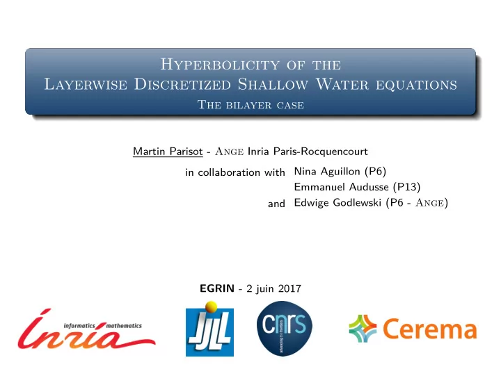
Hyperbolicity of the Layerwise Discretized Shallow Water equations The bilayer case Martin Parisot - Ange Inria Paris-Rocquencourt in collaboration with Nina Aguillon (P6) Emmanuel Audusse (P13) Edwige Godlewski (P6 - Ange ) and EGRIN - 2 juin 2017

Introduction Layerwise Discretized Shallow Water model Layerwise Discretized Shallow Water model: [Audusse, Bristeau, Perthame and Sainte-Marie’11] for i ∈ [ [1 , L ] ]  = [ G ] i + 1 / 2  + ∂ x ( h i u i ) + ∂ y ( h i v i )  ∂ t h i   i − 1 / 2   � � = − gh i ∂ x B + [ uG ] i + 1 / 2 i + g h i u 2 ( SW L ) ∂ t ( h i u i ) + ∂ x 2 h i h + ∂ y ( h i u i v i ) i − 1 / 2    � �  = − gh i ∂ y B + [ vG ] i + 1 / 2  i + g h i v 2  ∂ t ( h i v i ) + ∂ x ( h i v i u i ) 2 h i h + ∂ y i − 1 / 2 � with h i = α i h and α i = 1. i η u 5 ζ 11 / 2 h 5 G 9 / 2 u 4 ζ 9 / 2 h 4 h u ( z ) G 7 / 2 ζ 7 / 2 u 3 h 3 g G 5 / 2 ζ 5 / 2 u 2 h 2 G 3 / 2 ζ 3 / 2 u 1 h 1 B ζ 0 [Audusse, Bristeau, Pelanti and Sainte-Marie’11] with variable density. [Bristeau, Guichard, Di Martino and Sainte-Marie’16] with viscous terms. [Fernandez-Nieto, Parisot, Penel and Sainte-Marie] with non-hydrostatic terms. Martin PARISOT EGRIN 2017 Layerwise Discretized model 2 / 14

Introduction Layerwise Discretized Shallow Water model Layerwise Discretized Shallow Water model: [Audusse, Bristeau, Perthame and Sainte-Marie’11]  + ∂ x ( h 1 u 1 ) = 0 ∂ t h 1   � � 1 + g h 1 u 2 2 h 2 ( SW 1 ) ∂ t ( h 1 u 1 ) + ∂ x = 0 1   ∂ t ( h 1 v 1 ) + ∂ x ( h 1 v 1 u 1 ) = 0 η ζ 3 / 2 u ( z ) h 1 u 1 h g B ζ 0 � � Strictly hyperbolic equations u 1 − gh 1 u 1 + gh 1 u 1 Admissible shock define to ensure the mechanical � � energy dissipation : E = h 1 + g u 2 1 + v 2 2 h 2 2 1 1 �� u 2 � � 1 + v 2 x 1 ≤ 0 ∂ t E + ∂ x + gh 1 h 1 u 1 2 Dambreak SW 1 Martin PARISOT EGRIN 2017 Layerwise Discretized model 2 / 14

Introduction Layerwise Discretized Shallow Water model Layerwise Discretized Shallow Water model: [Audusse, Bristeau, Perthame and Sainte-Marie’11]   + ∂ x ( h 1 u 1 ) + ∂ x ( hu ) = 0 ∂ t h 1 = − G 3 / 2 ∂ t h   � � u 2 � 2 h 2 �       + g u 2 + �   ∂ t h 2 + ∂ x ( h 2 u 2 ) = G 3 / 2 ∂ t ( hu ) + ∂ x h = 0   ( SW 2 )    � �     1 + g  h 1 u 2 u + ∂ x ( � uu ) = 0 h 1 = h 2   ∂ t � ∂ t ( h 1 u 1 ) + ∂ x 2 h 1 h = − u 3 / 2 G 3 / 2 � � u 3 / 2 = u 1 + u 2 ∂ t ( hv ) + ∂ x ( h ( uv + � v )) = 0 ⇔ u � 2 + g h 2 u 2   2 ∂ t ( h 2 u 2 ) + ∂ x 2 h 2 h = u 3 / 2 G 3 / 2     ∂ t � v u ∂ x v + u ∂ x � v = 0 + � v 3 / 2 = v 1 + v 2       u = u 1 + u 2 u = u 2 − u 1 ∂ t ( h 1 v 1 ) + ∂ x ( h 1 v 1 u 1 ) = − v 3 / 2 G 3 / 2 2     �   2 2     v = v 1 + v 2 v = v 2 − v 1 ∂ t ( h 2 v 2 ) + ∂ x ( h 2 v 2 u 2 ) = v 3 / 2 G 3 / 2 � 2 2 η u 2 h 2 u h u ( z ) h g u � G 3 / 2 u 1 h 1 ζ 0 B [Teshukov’07, Richard and Gavrilyuk’12] shear model. [Castro and Lannes’14] with non-hydrostatic terms. Martin PARISOT EGRIN 2017 Layerwise Discretized model 2 / 14

Introduction Layerwise Discretized Shallow Water model Bi-layer model: Full-Euler model:  ∂ t h + ∂ x ( hu ) = 0 ,   � � ��   u 2 + g + ∂ x ( ρ u ) = 0 , ∂ t ρ hu 2 + h    � �  ∂ t ( hu ) + ∂ x 2 h = 0 , �    ρ u 2 + p ∂ t ( ρ u ) + ∂ x = 0 , ∂ t � u + ∂ x ( � uu ) = 0 ,    ∂ t ( ρ e ) + ∂ x (( ρ e + p ) u ) = 0 ,   ∂ t ( hv ) + ∂ x ( h ( uv + � v )) = 0 ,   u �    ∂ t ( ρ v ) + ∂ x ( ρ uv ) = 0 , ∂ t � v u ∂ x v + u ∂ x � v = 0 + � Admissible shock define to ensure Admissible shock define to ensure the entropy dissipation : the mechanical energy dissipation : � v 2 � + g ∂ t η + ∂ x ( η u ) ≤ 0 E = h u 2 + � u 2 + v 2 + � 2 h 2 2 �� � � u 2 + 3 � u 2 + v 2 + � v 2 ≤ 0 ∂ t E + ∂ x + gh hu + hv � v � u 2 1D analogous to the full-Euler equations except at the shock . Martin PARISOT EGRIN 2017 Layerwise Discretized model 3 / 14

Introduction Layerwise Discretized Shallow Water model Bi-layer model: Full-Euler model:  ∂ t h + ∂ x ( hu ) = 0 ,   � � ��   u 2 + g + ∂ x ( ρ u ) = 0 , ∂ t ρ hu 2 + h    � �  ∂ t ( hu ) + ∂ x 2 h = 0 , �    ρ u 2 + p ∂ t ( ρ u ) + ∂ x = 0 , ∂ t � u + ∂ x ( � uu ) = 0 ,    ∂ t ( ρ e ) + ∂ x (( ρ e + p ) u ) = 0 ,   ∂ t ( hv ) + ∂ x ( h ( uv + � v )) = 0 ,   u �    ∂ t ( ρ v ) + ∂ x ( ρ uv ) = 0 , ∂ t � v u ∂ x v + u ∂ x � v = 0 + � Admissible shock define to ensure Admissible shock define to ensure the entropy dissipation : the mechanical energy dissipation : � v 2 � + g ∂ t η + ∂ x ( η u ) ≤ 0 E = h u 2 + � u 2 + v 2 + � 2 h 2 2 �� � � u 2 + 3 � u 2 + v 2 + � v 2 ≤ 0 ∂ t E + ∂ x + gh hu + hv � v � u 2 1D analogous to the full-Euler equations except at the shock . 2D NOT analogous : non-conservative products, coalescence, resonance. Martin PARISOT EGRIN 2017 Layerwise Discretized model 3 / 14

1D bilayer model Hyperbolicity and waves patterns 1D Bi-layer model:    ∂ t h + ∂ x ( hu ) = 0 ,  h  � � �� u 2 + g hu 2 + h ∂ t ( hu ) + ∂ x = 0 ,   � 2 h We set U = hu   u � ∂ t � u + ∂ x ( � uu ) = 0 , Proposition : hyperbolicity of (1 D − SW 2 ) For physical solution, i.e. h > 0, the 1D bilayer model ( SW 2 ) is strictly hyperbolic . More precisely, the eigenvalues are given by � � u 2 u 2 . gh + 3 � gh + 3 � λ L = u − < λ ∗ = u < λ R = u + In addition, the λ L -wave and the λ R -wave are genuinely nonlinear , whereas the λ ∗ -wave is linearly degenerate . λ L ( U L ) λ L ( U L ∗ ) u ∗ σ R U L U L ∗ U R ∗ U R x Martin PARISOT EGRIN 2017 Layerwise Discretized model 4 / 14

1D bilayer model The 1D Riemann problem Proposition : admissible shock of (1 D − SW 2 ) We denote by σ k the speed of the λ k -shock. Assuming that the water depth h is positive, the following properties are equivalent: � u 2 � i) The mechanical energy E = g 2 h 2 + h u 2 + � is decreasing through a shock, i.e. 2 �� � � u 2 + 3 � u 2 − σ k [ E ] + + gh hu < 0 . 2 ii) the shock is compressive , i.e. we have � h 2 � � � � hu 2 � � hu 3 � � u 2 � � � h 2 u u 2 u − σ k + > 0 or − σ k + < 0 or − σ k h � + h � > 0 . iii) the Lax entropy condition is satisfied λ L ( U L ∗ ) < σ L < λ L ( U L ) λ R ( U R ) < σ R < λ R ( U R ∗ ) . and Remark : It is NOT a corollary of the classical theorem [Godlewsli, Raviart’96] since the mechanical energy E (acting as the mathematical entropy) is not a convexe function of the conserved variable U . Martin PARISOT EGRIN 2017 Layerwise Discretized model 5 / 14

1D bilayer model The 1D Riemann problem Theorem : Riemann problem of (1 D − SW 2 ) � u L ) t ∈ R ∗ + × R 2 U L = ( h L , u L , � if x < 0 , Consider the initial condition U (0 , x ) = u R ) t ∈ R ∗ + × R 2 U R = ( h R , u R , � if x ≥ 0 . If the following condition is fulfilled : u R − u L < µ r ( U L ) + µ r ( U R ) with �� � � � u 2 u 2 + gh 1 + 3 � 3 µ r ( U ) = gh + 3 � log u � gh + � gh 3 � u + × R )) 3 to the 1D Riemann problem then there exists a unique selfsimilar solution U ∈ ( L ∞ ( R ∗ ( SW 2 ) satisfying the mechanical energy dissipation . In addition the water depth h is strictly positive for all ( t , x ) ∈ R + × R . h L ∗ p L ∗ = p R ∗ h L Sketch of proof : • Determine the rarefaction and shock curves. 1 u L ∗ = u R ∗ 2 Conclude by monotony. h R h R ∗ Martin PARISOT EGRIN 2017 Layerwise Discretized model 6 / 14

2D bilayer model Hyperbolicity and waves patterns 2D Bi-layer model:    ∂ t h + ∂ x ( hu ) = 0 , h  � � u 2 � 2 h 2 �  + g   u 2 + �  ∂ t ( hu ) + ∂ x = 0 ,   h hu      u We set V = � ∂ t � u + ∂ x ( � uu ) = 0 ,        hv  ∂ t ( hv ) + ∂ x ( h ( uv + � u � v )) = 0 ,   v � ∂ t � v + � u ∂ x v + u ∂ x � v = 0 , Proposition : hyperbolicity of (2 D − SW 2 ) For physical solution, i.e. h > 0, the 2D bilayer model ( SW 2 ) is hyperbolic . More precisely, the eigenvalues are given by � � u 2 u 2 . λ L = u − gh + 3 � γ L = u −| � u | λ ∗ = u γ R = u +| � u | λ R = u + gh + 3 � < ≤ ≤ < In addition, the λ L -wave and the λ R -wave are genuinely nonlinear , whereas the γ L -wave, λ ∗ -wave and γ R -wave are linearly degenerate . λ L ( V L ) λ L ( V L ∗ ) γ L γ R σ R λ ∗ V L V L 1 V L 2 V R 2 V R 1 V R x Martin PARISOT EGRIN 2017 Layerwise Discretized model 7 / 14