http://ecosequestrust.org/GAMA resilience.io programme Global - PowerPoint PPT Presentation
http://ecosequestrust.org/GAMA resilience.io programme Global Update Global Update Preliminary outcomes of the agent-based modelling and resource network optimisation for the WASH sector in GAMA, Ghana Resilience.IO platform Harry
http://ecosequestrust.org/GAMA
resilience.io programme
Global Update
Global Update
Preliminary outcomes of the agent-based modelling and resource network optimisation for the WASH sector in GAMA, Ghana Resilience.IO platform Harry Triantafyllidis, Xiaonan Wang, Rembrandt Koppelaar and Koen H. van Dam Department of Chemical Engineering, Imperial College London, UK IIER – Institute for Integrated Economic Research 21 January 2016
Outline Introduction and context (Xiaonan Wang) • WASH use case 1 • Role of modelling and simulation • Agent-based modelling (Xiaonan Wang, Koen H. van Dam) • What and why • Applications in GAMA WASH simulation • Optimisation (Harry Triantafyllidis) • What and why • Preliminary/illustrative outcomes Use Case 1 • Towards the final model for the WASH sector in GAMA (Rembrandt Koppelaar) • Next steps • Interviews and review of use cases • Visual presentation • Discussion • 2
Introduction and context Speaker: Dr Xiaonan Wang 3
WASH Challenges – Use case 1 Three use cases were selected previously First focus on Use Case 1: Assess outcomes of ongoing WASH projects and gaps towards meeting macro-level targets for planning Input - Capacities and time frame - Calculate combined Model use effect of on-going projects of all ongoing projects when fully completed to - Targets and goals from targets local, national policies and - Estimate gaps remaining international agreements Projects & Targets - 5 to 20 years of - Costs/benefits from successful completion population, economic - Additional effort and status, and migration possibilities to meet - Socio-economic targets Output Scenarios scenarios 4
Approach: linking ABM and RTN Idea: use a simulation model of a synthetic population to experiment with different scenarios to generate demand profiles , which can then be used to optimise the technologies and networks with key performance metrics 5
Agent-based model of WASH sector in GAMA Speaker: Dr Xiaonan Wang, Dr Koen H. van Dam 6
Definition of agent-based modelling environment Agent-based modelling agent is a computational method that enables a researcher to state create, analyze, and experiment with models composed of agents that interact within an environment. behaviour (Nigel Gilbert, 2007) 7
Purpose of the model Stage 3 Provide long-term socio- economic scenarios Stage 2 Estimate demand for water resources based on activities of the population Stage 1 Simulate population of GAMA 8
Agent activities (example) AP i = {( ACT j , MDT j , SD j , PD j )} : Activity j ACT j : Mean departure time MDT j : Standard deviation SD j : Probability of departure PD j (Activities depend on agent characteristics) 9
Agent characteristics Agent 9
Synthetic population (1/2) Agents are generated in a stochastic process based on real data collected for GAMA, leading to a representative synthetic population (~0.1% of real population) Socio-economic Gender (male or female) Age (0-14 years or 15+) Work force status (Employed / Not active or unemployed) Income status (Low income / Medium income / High income) Spatial Home location (point in district/MMDA) Work location , for those economically active, based on distance from home 11
Synthetic population (2/2) Access to infrastructure Drinking water (private pipe access / public tap or stand pipe / protected decentralised source / unprotected decentralised source / tanker and vendor provided / sachet water / bottled water) simplified to private/non- private access Non-drinking water (private pipe access / public tap or stand pipe / protected decentralised source / unprotected decentralised source / tanker and vendor provided) simplified to private/non-private access Toilet (Water closet / Kumasi VIP / Pit Latrine / Public Toilet / Bucket or Pan Latrine / No facilities) Household demands are dependent on: Access to infrastructure Income level Time of day (i.e. activities) 12
First model (shown in August 2015 webinar) 13
Model development – Progress update Expansions Work in progress: implemented: Non-residential Detailed water use and demands flow from human Pipelines and sewage activities (modelled) flows Waste water flow Toilet use Commuting (basic) Commuting (detailed) Data collection per Incorporate long-term MMDA population and economic scenarios 13
Screenshot agent-based simulation 15
Screenshot agent-based simulation time tick 240 time tick 60 time tick 120 dense agent population 16
Example outcomes Drinking water demand profile per MMDA over 24 hour period Total potable water demands (annual): 31.9 million m 3 these demands feed into the RTN for optimisation 17
Example outcomes Waste water profile per MMDA over 24 hour period Total waste water generation (annual): 814.1 million m 3 these demands feed into the RTN for optimisation 18
Resource-Technology Network optimisation Speaker: Dr Harry Triantafyllidis 19
Approach: linking ABM and RTN Idea: use a simulation model of a synthetic population to experiment with different scenarios to generate demand profiles , which can then be used to optimise the technologies and networks with key performance metrics 20
Preparing the data Current technology in place Demands from ABM Technical specifications Flow costs, capital expenditure, operational costs, import values, emissions Pipe network (?) across districts MMDAs coordinates 21
How the optimization works Production rates – satisfy demands Technology balance – investments Import resources? Resource surplus – better to flow it around or build infrastructure? Minimize cost/CO 2 emissions while treating the network as a whole 22
Technological infrastructure - potable water 23
Technological infrastructure - wastewater 24
Resources in network raw source water 1. electricity 2. labour hours 3. Potable potable water 4. water sludge 5. Labour hours electricity pot distributed water 6. carbon dioxide 7. influent wastewater 8. Raw source water raw waste water 9. 10. drink water sachet 11. treated effluent 12. influent faecal sludge 25
Characteristics of test model 15 MMDAs 2-year simulation (not fixed) with ability to split a single day for 5 periods, each reflecting different demands 17 tech types, 12 resources Pipe connections Pre-allocated tech units on base year (2010) Optimize capex/opex/CO 2 Satisfy % of demands in potable water and treated waste water 26
Preliminary outcomes of use case 1 27
Example – USE CASE 1 - work in progress Detailed implementation: The formulated model has 5,191 constraints and 36,455 variables 20% of demands in potable water and treated waste water with existing infrastructure + investments: KPI('capex'.2010) = ~16,8 billion USD KPI('opex'.2010) = ~ 36 million USD KPI('CO 2 '.2010) = ~8k tons / m 3 70% : KPI('capex'.2011) = 0 USD KPI('opex'.2011) = ~ 127 million USD KPI('CO 2 '.2011) = ~ 29k tons / m 3 28
Automated Visualized output MMDA’s on map • Associated optimal flows • Geo-localized • Connectivity • Bandwidth of flow visualized with the width of each edge • MMDA’s size scaling up with demands 29
Provide insights under various input scenarios and for specific targets Implement current status of infrastructure and experiment with costs / alternative tech types Insight where to build new infrastructure for cost reduction Let the model figure out from scratch the optimal allocation of the network and associated resource flows Employ long-term provision depending on different future policies or needs (ABM-RTN re-feed) Project technical importance of any component (predict impact of flaws / breakdowns in network) Calculate environmental impact of decisions! 30
Next steps use cases and stakeholder engagement Speaker: Rembrandt Koppelaar 31
Next Steps Refine and improve current Use Case 1, build functionality for • Use Case 2 (improved water) and 3 (toilet use) Refine technology selection for calculation CAPEX and OPEX • Add functionality for water and sewage pipe system expansion • Simulation of toilet use during the day • Integrate financial charges for pipe connections, water use and • toilet use by simulated population based on PURC tariffs, public, private fees How much does the infrastructure use cost the population, and what • revenues are generated per MMDA? 32
Next Steps Build capability to include scenarios for population and • household demographics change to 2030 What infrastructure is needed and what is the cost to respond to • demographic changes and associated water demands, toilet usage, and wastewater treatment needs? Include rainfall patterns and agricultural water demands • How do changes in rainfall and affect water needs, and what would be the • implication of increased irrigation on (waste)water treatment? 33
Recommend
More recommend
Explore More Topics
Stay informed with curated content and fresh updates.
