
How not to build a Model: Coupling Cloud Parameterizations Across Scales Andrew Gettelman, NCAR
All models are wrong. But some are useful. -George E. P. Box, 1976 (Statistician) “The Treachery of Images”, René Magritte, 1928
How NOT to build a model: Outline • Philosophy of Integrating Parameterizations • Optimization of Parameterizations (‘Tuning’) • Scale issues • Numerical considerations (clipping and stability) • Developing a physical parameterization suite across scales • CESM development example
Developers view of an ESM Dynamical CorePlumbing that Connects Them Parameterizations (Tendency Generators)
A Better View Connections Dynamical core Parameterizations (Tendency Generators) Microphysics Condensation Deep Convection /Fraction
How do we develop a model? • Parameterization development • Evaluation against theory and observations • Constrain each process & parameterization to be physically realistic • Conservation of mass and energy • Other physical laws • Connect each process together (plumbing) • Coupled: connect each component model • Global constraints • Make the results match important global or emergent properties of the earth system • “Training” (optimization, tuning)
Why doesn’t it work? • Process rates are uncertain at a given scale “all models are wrong…” (uncertainty v. observations) • Problems with the dynamical core • Problems connecting processes • Each parameterization is it’s own ‘animal’ & performs differently with others (tuning = training, limits) Each parameterization needs to contribute to a self consistent whole
Stages of Optimization (Training) Parameterization Process Component (land) Component (ocean) Earth System Component (atmos)
Problems with parameterizations • Need to ensure (enforce) mass and energy conversion • Represent sub-grid scale variability • This changes with time and space scales • Potentially a critical issue • Couple to other processes • Example: • Multiple cloud schemes (deep conv, condensation, micro) • Pass condensation to cloud microphysics • Get advective terms and dynamical (U,V) and radiative (T) forcing from dynamical core • Model state is a push-pull interaction
How do we optimize parameterizations? • Basic level: adjust (‘clip’) process rates • Conservation & numerics issue • Can also modify the ‘uncertain’ parts of parameterizations • Uncertainty comes from imperfect observations • Scale dependent • Also problems with coupling (push-pull) • Implicitly: adjust the ‘least certain’ • Least certain processes • Least certain observations
Scale issues Example: off line sensitivity of cloud microphysics rain rate to time step, with a constant condensation rate: Rain rates are stable, but LWP is not. Is this surprising? (more condensation per timestep) Is the parameterization wrong, or coupling to rest of model? Gettelman & Morrison, 2014, in press, J. Clim
Numerics: Sedimentation Levels v. Critical Timestep Figure: maximum timestep for satisfying CFL condition with different updraft speeds and fall speeds for rain (5m/s) • 1800 s GCM Timesteps • If rain falls at 1-5 m/s, then in 1 timestep it crosses several levels • CFL problem for sedimentation • Control for this in microphysics (sub-steps)
Numerical clipping • Can ‘run out of water’ with long time steps • Process rates non- linear: lots of condensation = more autoconversion • Shorter time steps yield a different solution
Coupling to condensation • Similar issues occur with condensation itself, and coupling with macrophysics
Physical Parameterization Suites • Community Earth System Model • Atmospheric component • Goals: Simulate and Predict the Earth System • Developmental model: enable science • We can still break things • Current status: releasing a model for CMIP6 • CESM2, CAM6 is the atmosphere component • Ongoing development: “across scales” • Pushing to work across weather to climate • Need to develop parameterizations across scales • Also: COUPLE parameterizations (sub-grid scale important)
The CAM family Model CAM3 CAM4 CAM5 (CAM5.3) CAM6 CCSM3 CCSM4 CESM1.0 (CESM1.2) CESM2 Release Jun 2004 Apr 2010 Jun 2010 (Nov 2012) January 2017 Gettelman-Morrison Microphysics Rasch-Kristjansson (1998) Rasch-Kristjansson (1998) Morrison-Gettelman (2008) (2015) MG2 Deep Convection Zhang-McFarlane (1995) ZM, Neale et al. (2008) ZM, Neale et al. (2008) ZM, Neale et al. (2008) PBL Holtslag-Boville (1993) Holtslag-Boville (1993) Bretherton et al (2009) CLUBB: Bogenschutz et al 2013 Shallow Hack (1994) Hack (1994) Park et al. (2009) Convection Macrophysics Rasch-Kristjansson (1998) Rasch-Kristjansson (1998) Park et al. (2011) Radiation Collins et al. (2001) Collins et al. (2001) Iacono et al. (2008) Iacono et al. (2008) 3 MODE Modal Aerosol 4 MODE Modal Model Aerosol Model Aerosols Bulk Aerosol Model Bulk Aerosol Model BAM Ghan et al. (2011) Ghan et al. (2011) Finite Volume//Spectral Dynamics Spectral Finite Volume Finite Volume Element (High Res) = New parameterization/dynamics
Community Atmosphere Model (CAM4) CCSM4: IPCC AR5 version (Neale et al 2010) Finite Volume Cartesian Dynamics Collins (CAMRT) Surface Fluxes Precipitation Radiation Bulk, Prescribed Boundary Layer Aerosols Holtslag-Boville Clouds (A l ), Condensate (q v , q c ) Shallow Convection Condensation: Zhang et al Microphysics 1 Moment Hack Detrained q c ,q i Rasch-Kristjannson Slingo, Cloud Fraction Deep Convection Clouds & Condensate: Klein-Hartmann T, A deep , A sh Zhang & McFarlane A = cloud fraction, q=H 2 O, re=effective radius (size), T=temperature (i)ce, (l)iquid, (v)apor
Community Atmosphere Model (CAM5) CAM5.1-5.3: IPCC AR5 version (Neale et al 2010) ‘New’ Finite Volume Cartesian Dynamics RRTMG Surface Fluxes 3-Mode Liu, Ghan et al Precipitation Radiation Boundary Layer Aerosols Bretherton A, q c , q i , q v Crystal/Drop Mass, & Park re i , re l Number Conc Activation Microphysics Shallow Convection 2 Moment Park & Detrained q c ,q i Morrison & Gettelman Clouds (A l ), Bretherton Condensate (q v , q c ) Ice supersaturation Diag 2-moment Precip Macrophysics Deep Convection Clouds & Condensate: T, A deep , A sh Park et al: Equil PDF Zhang & McFarlane A = cloud fraction, q=H 2 O, re=effective radius (size), T=temperature (i)ce, (l)iquid, (v)apor
Community Atmosphere Model (CAM6) CMIP6 model Finite Volume Cartesian Dynamics Surface Fluxes 4-Mode Liu, Ghan et al Precipitation Crystal/Drop A, q c , q i , q v Activation re i , re l Radiation Aerosols Deep Convection Mass, Zhang- Number Conc Sub-Step McFarlane Microphysics 2 Moment Morrison & Gettelman Clouds (A l ), Condensate (q v , q c ) Ice supersaturation Unified Turbulence Prognostic 2-moment Precip Clouds & Condensate: T, A deep , A sh CLUBB A = cloud fraction, q=H 2 O, re=effective radius (size), T=temperature (i)ce, (l)iquid, (v)apor
Community Atmosphere Model (0.25°) Working on this as an option Spectral Element Cubed Sphere: Variable Resolution Mesh Dynamics Surface Fluxes 4-Mode Liu, Ghan et al Precipitation Crystal/Drop A, q c , q i , q v Activation re i , re l Radiation Aerosols Deep Convection Mass, Zhang- Number Conc Sub-Step McFarlane Microphysics 2 Moment Morrison & Gettelman Clouds (A l ), Condensate (q v , q c ) Ice supersaturation Unified Turbulence Prognostic 2-moment Precip Clouds & Condensate: T, A deep , A sh CLUBB A = cloud fraction, q=H 2 O, re=effective radius (size), T=temperature (i)ce, (l)iquid, (v)apor
Community Atmosphere Model (CAM6.X) Now in development: Sub-columns Spectral Element Cubed Sphere Dynamics 4-Mode Surface Fluxes Liu, Ghan et al Averaging Precipitation Crystal/Drop A, q c , q i , q v Activation re i , re l Radiation Aerosols Mass, Sub-Step Number Conc Microphysics 2 Moment Morrison & Gettelman Clouds & Condensate: Unified Turbulence T, A deep , A sh Ice supersaturation Prognostic 2-moment Precip CLUBB Sub Columns A = cloud fraction, q=H 2 O, re=effective radius (size), T=temperature (i)ce, (l)iquid, (v)apor
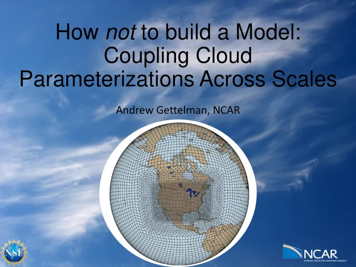
Regional Climate modeling Critical for testing parameterizations • Regional Climate Framework • Refine over narrow region, or whole ocean basin Dynamics seems to work. Testing whether the physics works now. Baseline: Coterminous United States (CONUS) Also: tools to build refinement for anywhere. 100km 12km (hydrostatic) 100km 3km (non-hydrostatic)
CESM: High resolution Mesh Biases v. ERA-I DJF Precipitation Climatology Reduced biases at high resolution, especially orographic precip 25km 100km (%) Re-gridded to 100km
Philosophy of Interactions • Consistency across/between parameterizations is key • Cannot just pick from a buffet • Couple parameterizations effectively • ‘simple’ parameterizations • ‘fewer’ parameterizations (less complex linkages) • Optimize parameterizations together • Flexibility for sub-grid variability • What is ‘sub-grid’ may change with resolution • Make sure representations are valid across scales • Build in capability to test across scales from weather to climate • Climate felt through weather (need key detailed processes) • Weather should obey conservation • Unified FRAMEWORK (not necessarily a single model)
Recommend
More recommend