Homework 5 Due Tuesday Oct 26 CLRS 14-2.2 (rb tree black height) - PDF document
Homework 5 Due Tuesday Oct 26 CLRS 14-2.2 (rb tree black height) CLRS 14-2.3 (rb tree depth) CLRS 14-1 (point of maximum overlap) CLRS 15.1-4 (assembly line space requirement) 1 Chapter 15: Dynamic programming Dynamic programming
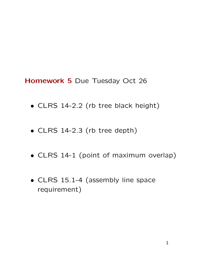
Homework 5 Due Tuesday Oct 26 • CLRS 14-2.2 (rb tree black height) • CLRS 14-2.3 (rb tree depth) • CLRS 14-1 (point of maximum overlap) • CLRS 15.1-4 (assembly line space requirement) 1
Chapter 15: Dynamic programming Dynamic programming is a method for designing efficient algorithms for recursively solvable problems with the following properties: 1. Optimal Substructure: An optimal solution to an instance contains an optimal solution to its sub-instances. 2. Overlapping Subproblems: The number of subproblems is small so during the recursion same instances are referred to over and over again. 2
Four steps in solving a problem using the dynamic programming technique 1. Characterize the structure of an optimal solution 2. Recursively define the value of an optimal solution 3. Compute the value of an optimal solution in a bottom-up fashion 4. Construct an optimal solution from computed information 3
The Problems to be Studied 1. Assembly-line Scheduling · · · the problem of finding the best choices for stations in two assembly lines 2. Matrix-chain Multiplication · · · the problem of finding the ordering of matrix-multiplication that minimizes the total number of scalar multiplications. 3. Longest Common Subsequence · · · the problem of finding the longest sequence that appears commonly in a pair of strings. 4. Optimal Binary Tree · · · Finding the arrangement of nodes that minimizes the average search time 4
I. Assembly-line Scheduling Assume you own a factory for car assembling. The car you will be producing has n parts and the parts need to be put on the chassis in a fixed order. There are two different assembly lines. Each line consists of n stations, where for each i , 1 ≤ i ≤ n , the i th station is for putting the i th part. The time required for a station varies. When a chassis leaves a station for the next part it is possible to move the chassis to the other line, but that takes extra time depending on which station the chassis is at the moment. Also, each line has a certain entry time and an exit time. What are the choice of the stations so as to minimize the production time? 5
Line 1 3 8 6 3 4 2 4 2 1 2 1 2 4 enter finish 1 1 3 6 3 3 4 Line 2 5 10 2 2 5 3 6
How about testing all possible paths? 7
How about testing all possible paths? There are 2 n possible paths. For large n exhaustive search is not going to work. There is an O ( n ) -time solution to this problem. The trick is to find the fastest path to each station. 8
Mathematical Formulation For each i ∈ { 1 , 2 } and for each j , 1 ≤ j ≤ n , let S i,j denote the j th station in line i . For each i ∈ { 1 , 2 } , define the following quantities: • e i is the entry time into line i . • x i is the exit time from line i . • For each j , 1 ≤ j ≤ n − 1, t i,j is the time that it takes for moving from S i,j to S 3 − i,j +1 . • For each j , 1 ≤ j ≤ n , a i,j is the time required for station S i,j . 9
Step 1: Characterizing structure of the optimal solution To compute the fastest assembly time, we only need to know the fastest time to S 1 ,n and the fastest time to S 2 ,n , including the assembly time for the n th part. Then we choose between the two exiting points by taking into consideration the extra time required, x 1 and x 2 . To compute the fastest time to S 1 ,n we only need to know the fastest time to S 1 ,n − 1 and to S 2 ,n − 1 . Then there are only two choices... 10
Step 2: A recursive definition of the values to be computed For each i ∈ { 1 , 2 } and for each j , 1 ≤ j ≤ n , let f i [ j ] be the fastest possible time to get to station S i,j , including the assemble time at S i,j . Let f ∗ be the fastest time for the entire assembly. Then f ∗ = min( f 1 [ n ] + x 1 , f 2 [ n ] + x 2 ). For all j , 2 ≤ j ≤ n , we have f 1 [ j ] = min( f 1 [ j − 1] + a 1 ,j , f 2 [ j − 1] + t 2 ,j − 1 + a 2 ,j ) and f 2 [ j ] = min( f 1 [ j − 1] + t 1 ,j − 1 + a 1 ,j , f 2 [ j − 1] + a 2 ,j ). 11
Step 3: Computing the fastest time First, set f 1 [1] = e 1 + a 1 , 1 and f 2 [1] = e 2 + a 1 , 2 . Then, for j ← 2 to n , compute f 1 [ j ] as min( f 1 [ j − 1] + a 1 ,j , f 2 [ j − 1] + t 2 ,j − 1 + a 1 ,j ) and f 2 [ j ] as min( f 1 [ j − 1] + t 1 ,j − 1 + a 2 ,j , f 2 [ j − 1] + a 2 ,j ). Finally, compute f ∗ as min( f 1 [ n ] + x 1 , f 2 [ n ] + x 2 ). 12
Step 4: Computing the fastest path For each i ∈ { 1 , 2 } , and for each j , 2 ≤ j ≤ n , compute as l i [ j ] as the choice made for f i [ j ] (whether the first or the second term gives the minimum). Also, compute the choice for f ∗ as l ∗ . Then we have only to trace back the choices to find the fastest path. 13
Fastest - Way ( a, t, e, x, n ) 1: f 1 [1] ← e 1 + a 1 , 1 2: f 2 [1] ← e 2 + a 1 , 2 3: for j ← 2 to n do { 4: if f 1 [ j − 1] + a 1 ,j ≤ f 2 [ j − 1] + t 2 ,j − 1 + a 1 ,j 5: then { f 1 [ j ] ← f 1 [ j − 1] + a 1 ,j 6: l 1 [ j ] ← 1 } else { f 1 [ j ] ← f 2 [ j − 1] + t 2 ,j − 1 + a 1 ,j 7: l 1 [ j ] ← 2 } 8: 9: if f 2 [ j − 1] + a 2 ,j ≤ f 1 [ j − 1] + t 1 ,j − 1 + a 2 ,j 10: then { f 2 [ j ] ← f 2 [ j − 1] + a 2 ,j 11: l 2 [ j ] ← 2 } 12: else { f 2 [ j ] ← f 1 [ j − 1] + t 1 ,j − 1 + a 2 ,j 13: l 2 [ j ] ← 1 } 14: if f 1 [ n ] + x 1 ≤ f 2 [ n ] + x 2 then { f ∗ ← f 1 [ n ] + x 1 15: l ∗ ← 1 } 16: 17: else { f ∗ ← f 2 [ n ] + x 2 l ∗ ← 2 } 18: 14
Example j 1 2 3 4 5 6 f 1 [ j ] 7 15 21 22 25 27 l 1 [ j ] 1 1 2 2 1 f 2 [ j ] 8 18 18 20 25 28 l 2 [ j ] 2 1 2 2 2 f ∗ = 31 and l ∗ = 1 Line 1 3 8 6 3 4 2 4 2 1 2 1 2 4 enter finish 1 1 3 6 3 3 4 Line 2 5 10 2 2 5 3 15
II. Matrix-Chain Multiplication Suppose that we need to compute the product M = A 1 · · · A n of matrices A 1 , . . . , A n . In the standard matrix multiplication, to compute the product of two matrices of dimension p × q and q × r , pqr scalar multiplications are needed. The multiplication over matrices is an associative operation. So, there are many different ways to compute the product. Use parentheses to describe the order. If the sizes of the matrix are not uniform, the cost of computing the product may be dependent on the order in which the matrices are multiplied. The matrix-chain multiplication problem is the problem of, given a sequence of matrices, finding the order of multiplications that minimizes the total cost. 16
Example Suppose we need to compute ABC , where A is 10 × 100, B is 100 × 10, and C is 10 × 100 How many operations for A ( BC ) ? 17
10 100 100 10 100 10 A B C 10,000 10,000 10 100 10 10 20,000 total 18
Parenthesization of Matrix Chain A chain of matrices is fully parenthesized if it is either a single matrix or the product of two fully parenthesized matrix products. How many different fully parenthesizations are there for ABCD ? 19
There are five: ( A ( B ( CD ))), ( A (( BC ) D )), (( A ( BC )) D ), (( AB )( CD )), and ((( AB ) C ) D ). Then how many are there for n matrices? 20
The Number of Full Parenthesizations For each n ≥ 1, let P ( n ) be the number of distinct full parenthesizations of a chain of n matrices. Then � 1 if n = 1, P ( n ) = � n − 1 k =1 P ( k ) P ( n − k ) if n ≥ 2. Solving this, we obtain P ( n ) = C ( n − 1), where 1 � 2 n � C ( n ) = n + 1 n 21
Redefining the Problem Using the concept of full parenthesization the problem can be redefined as follows: Given a list p = ( p 0 , p 1 , . . . , p n ) of positive integers, compute the optimal-cost full-parenthesization of any chain ( A 1 , A 2 , . . . , A n ), such that for all i , 1 ≤ i ≤ n , the dimension of the i th matrix is dimension p i − 1 × p i , where the cost is measured by the total number of scalar multiplications when the standard matrix multiplication is used. 22
Inefficiency of Brute-force Search One cannot use brute-force search to solve this problem, because 1 � 2 n � = Ω(4 n /n 3 / 2 ) . C ( n ) = n + 1 n However, there is a solution with O ( n 3 ) running time. 23
Step 1: Characterization of the structure The outermost pair of parentheses splits the matrix sequence into two. Suppose that the split is between A 1 , . . . , A k and A k +1 , . . . , A n . Then to evaluate the product via this split, we compute B ( k ) = A 1 · · · A k and C ( k ) = A k +1 · · · A n , then B ( k ) C ( k ). 24
Suppose the optimal cost of computing B ( k ) and C ( k ) is known for all k, 1 ≤ k ≤ n − 1. Then we can compute the optimal cost for the entire product by finding a k that minimizes “the optimal cost for computing B ( k )” + “the optimal cost for computing C ( k )” + p 0 p k p n . This suggests a bottom-up approach for computing the optimal costs. 25
Step 2: A recursive solution For each i , 1 ≤ i ≤ n , and each j , 1 ≤ i ≤ j ≤ n , let m [ i, j ] be the optimal cost for computing A i · · · A j . Then for all i , 1 ≤ i ≤ n , m [ i, i ] = 0 and for all i and j , 1 ≤ i < j ≤ n , m [ i, j ] is the minimum of m [ i, k ] + m [ k + 1 , j ] + p i − 1 p k p j , where i ≤ k ≤ j − 1 26
Step 3: Computing the optimal cost 1. For i = 1 , . . . , n , set m [ i, i ] = 0. 2. For ℓ ← 2 to n , and for all i and j such that j − i + 1 = ℓ , compute m [ i, j ]. 27
Recommend
More recommend
Explore More Topics
Stay informed with curated content and fresh updates.
