Homework 4. SDP Extensions of PCA/MDS Instructor: Yuan Yao Due: - PDF document

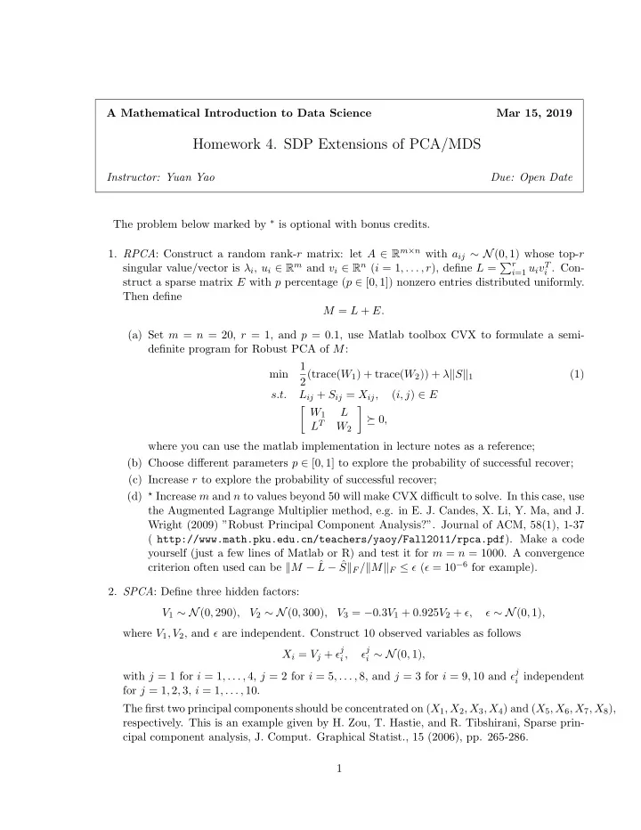
A Mathematical Introduction to Data Science Mar 15, 2019 Homework 4. SDP Extensions of PCA/MDS Instructor: Yuan Yao Due: Open Date The problem below marked by ∗ is optional with bonus credits. 1. RPCA : Construct a random rank- r matrix: let A ∈ R m × n with a ij ∼ N (0 , 1) whose top- r singular value/vector is λ i , u i ∈ R m and v i ∈ R n ( i = 1 , . . . , r ), define L = � r i =1 u i v T i . Con- struct a sparse matrix E with p percentage ( p ∈ [0 , 1]) nonzero entries distributed uniformly. Then define M = L + E. (a) Set m = n = 20, r = 1, and p = 0 . 1, use Matlab toolbox CVX to formulate a semi- definite program for Robust PCA of M : 1 2(trace( W 1 ) + trace( W 2 )) + λ � S � 1 min (1) s.t. L ij + S ij = X ij , ( i, j ) ∈ E � W 1 � L � 0 , L T W 2 where you can use the matlab implementation in lecture notes as a reference; (b) Choose different parameters p ∈ [0 , 1] to explore the probability of successful recover; (c) Increase r to explore the probability of successful recover; (d) ⋆ Increase m and n to values beyond 50 will make CVX difficult to solve. In this case, use the Augmented Lagrange Multiplier method, e.g. in E. J. Candes, X. Li, Y. Ma, and J. Wright (2009) ”Robust Principal Component Analysis?”. Journal of ACM, 58(1), 1-37 ( http://www.math.pku.edu.cn/teachers/yaoy/Fall2011/rpca.pdf ). Make a code yourself (just a few lines of Matlab or R) and test it for m = n = 1000. A convergence S � F / � M � F ≤ ǫ ( ǫ = 10 − 6 for example). criterion often used can be � M − ˆ L − ˆ 2. SPCA : Define three hidden factors: V 1 ∼ N (0 , 290) , V 2 ∼ N (0 , 300) , V 3 = − 0 . 3 V 1 + 0 . 925 V 2 + ǫ, ǫ ∼ N (0 , 1) , where V 1 , V 2 , and ǫ are independent. Construct 10 observed variables as follows X i = V j + ǫ j ǫ j i , i ∼ N (0 , 1) , with j = 1 for i = 1 , . . . , 4, j = 2 for i = 5 , . . . , 8, and j = 3 for i = 9 , 10 and ǫ j i independent for j = 1 , 2 , 3, i = 1 , . . . , 10. The first two principal components should be concentrated on ( X 1 , X 2 , X 3 , X 4 ) and ( X 5 , X 6 , X 7 , X 8 ), respectively. This is an example given by H. Zou, T. Hastie, and R. Tibshirani, Sparse prin- cipal component analysis, J. Comput. Graphical Statist., 15 (2006), pp. 265-286. 1

Homework 4. SDP Extensions of PCA/MDS 2 (a) Compute the true covariance matrix Σ (and the sample covariance matrix with n exam- ples, say n = 1000); (b) Compute the top 4 principal components of Σ using eigenvector decomposition (by Matlab or R); (c) Use Matlab CVX toolbox to compute the first sparse principal component by solving the SDP problem max trace(Σ X ) − λ � X � 1 s.t. trace( X ) = 1 X � 0 Choose λ = 0 and other positive numbers to compare your results with normal PCA; (d) Remove the first sparse PCA from Σ and compute the second sparse PCA with the same code; (e) Again compute the 3rd and the 4th sparse PCA of Σ and compare them against the normal PCAs. (f) ⋆ Construct an example with 200 observed variables which is hard to deal with by CVX. In this case, use the Augmented Lagrange Multiplier method by Allen Yang et al. (UC Berkeley) whose Matlab codes can be found at http://www.eecs.berkeley.edu/ ~yang/software/SPCA/SPCA_ALM.zip . 3. Protein Folding: Consider the 3D structure reconstruction based on incomplete MDS with uncertainty. Data file: http://yao-lab.github.io/data/protein3D.zip Figure 1: 3D graphs of file PF00018 2HDA.pdf (YES HUMAN/97-144, PDB 2HDA) In the file, you will find 3D coordinates for the following three protein families: PF00013 (PCBP1 HUMAN/281-343, PDB 1WVN),

Homework 4. SDP Extensions of PCA/MDS 3 PF00018 (YES HUMAN/97-144, PDB 2HDA), and PF00254 (O45418 CAEEL/24-118, PDB 1R9H). For example, the file PF00018 2HDA.pdb contains the 3D coordinates of alpha-carbons for a particular amino acid sequence in the family, YES HUMAN/97-144, read as VALYDYEARTTEDLSFKKGERFQIINNTEGDWWEARSIATGKNGYIPS where the first line in the file is 97 V 0.967 18.470 4.342 Here • ‘97’: start position 97 in the sequence • ‘V’: first character in the sequence • [ x, y, z ]: 3D coordinates in unit ˚ A . Figure 1 gives a 3D representation of its structure. Given the 3D coordinates of the amino acids in the sequence, one can computer pairwise distance between amino acids, [ d ij ] l × l where l is the sequence length. A contact map is defined to be a graph G θ = ( V, E ) consisting l vertices for amino acids such that and edge ( i, j ) ∈ E if d ij ≤ θ , where the threshold is typically θ = 5˚ A or 8˚ A here. Can you recover the 3D structure of such proteins, up to an Euclidean transformation (rotation and translation), given noisy pairwise distances restricted on the contact map graph G θ , i.e. given noisy pairwise distances between vertex pairs whose true distances are no more than θ ? Design a noise model (e.g. Gaussian or uniformly bounded) for your experiments. When θ = ∞ without noise, classical MDS will work; but for a finite θ with noisy mea- surements, SDP approach can be useful. You may try the matlab package SNLSDP by Kim-Chuan Toh, Pratik Biswas, and Yinyu Ye, downladable at http://www.math.nus.edu. sg/~mattohkc/SNLSDP.html .