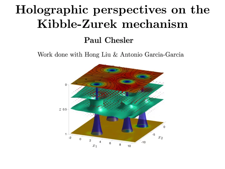
Holographic perspectives on the Kibble-Zurek mechanism z x 2 x 1 - PowerPoint PPT Presentation

Holographic perspectives on the Kibble-Zurek mechanism z x 2 x 1

What is the Kibble-Zurek mechanism? QFT with 2 nd order phase transition: • Example: superfluid • Symmetry group U (1) broken for T < T c . broken unbroken • Order parameter 6 = 0 for T < T c . • What happens when T is dynamic? ✏ ( t ) ⌘ 1 � T ( t ) . T c • Density of defects after quench: n ⇠ ⇠ − ( d − D ) .

What is the Kibble-Zurek mechanism? QFT with 2 nd order phase transition: • Example: superfluid • Symmetry group U (1) broken for T < T c . broken unbroken • Order parameter 6 = 0 for T < T c . • What happens when T is dynamic? ✏ ( t ) ⌘ 1 � T ( t ) . Box of T c superfluid • Density of defects after quench: at T > T c n ⇠ ⇠ − ( d − D ) .

What is the Kibble-Zurek mechanism? QFT with 2 nd order phase transition: • Example: superfluid • Symmetry group U (1) broken for T < T c . broken unbroken • Order parameter 6 = 0 for T < T c . • What happens when T is dynamic? ✏ ( t ) ⌘ 1 � T ( t ) . Box of T c superfluid • Density of defects after quench: at T > T c n ⇠ ⇠ − ( d − D ) . } ξ

What is the Kibble-Zurek mechanism? QFT with 2 nd order phase transition: • Example: superfluid • Symmetry group U (1) broken for T < T c . broken unbroken • Order parameter 6 = 0 for T < T c . • What happens when T is dynamic? ✏ ( t ) ⌘ 1 � T ( t ) . Box of T c superfluid • Density of defects after quench: at T > T c n ⇠ ⇠ − ( d − D ) . } ξ

Zurek’s estimate of correction length Critical slowing down • Critical exponents: ⇠ eq = ⇠ o | ✏ | − ν and ⌧ eq = ⌧ o | ✏ | − z ν . • Inevitable ∃ t freeze such that ∂τ eq � t = t freeze ∼ 1. � ∂ t broken unbroken − t freeze + t freeze • Characteristic scale: ⇠ freeze ≡ ⇠ eq ( t = t freeze ) .

The Kibble-Zurek scaling ψ ( t ) ∼ ✏ ( t ) β frozen t adiabatic − t freeze + t freeze • Assume linear quench: ✏ ( t ) = t/ ⌧ Q . ⇒ t freeze ∼ ⌧ ν z/ (1+ ν z ) ⇠ freeze ∼ ⌧ ν / (1+ ν z ) , . Q Q • Density of topological defects when condensate first forms: 1 ∼ ⌧ − ( d − D ) ν / (1+ ν z ) n KZ ∼ Q ⇠ d − D freeze

Motivational claims 1. Dynamics after + t freeze need not be adiabatic. • Adiabatic evolution only after t eq � t freeze . 2. No well-defined condensate until t eq . 3. Dynamics after T < T c responsible for KZ scaling. 4. ξ ( t eq ) � ξ freeze ) far fewer defects formed

Motivational claims 1. Dynamics after + t freeze need not be adiabatic. • Adiabatic evolution only after t eq � t freeze . 2. No well-defined condensate until t eq . 3. Dynamics after T < T c responsible for KZ scaling. 4. ξ ( t eq ) � ξ freeze ) far fewer defects formed excerpt from [Del Campo & Zurek] magnitude prediction usually overestimates the real density of defects ob- served in numerics. A better estimate is obtained by using a factor f , to multiply ˆ ξ in the above equations, where f ≈ 5 − 10 depends on the specific model. 29,31–35 Thus, while KZM provides an order-of-magnitude estimate

Motivational claims 1. Dynamics after + t freeze need not be adiabatic. • Adiabatic evolution only after t eq � t freeze . 2. No well-defined condensate until t eq . 3. Dynamics after T < T c responsible for KZ scaling. 4. ξ ( t eq ) � ξ freeze ) far fewer defects formed excerpt from [Del Campo & Zurek] magnitude prediction usually overestimates the real density of defects ob- served in numerics. A better estimate is obtained by using a factor f , to multiply ˆ ξ in the above equations, where f ≈ 5 − 10 depends on the specific model. 29,31–35 Thus, while KZM provides an order-of-magnitude estimate Employ holographic duality

Motivational claims 1. Dynamics after + t freeze need not be adiabatic. • Adiabatic evolution only after t eq � t freeze . 2. No well-defined condensate until t eq . 3. Dynamics after T < T c responsible for KZ scaling. 4. ξ ( t eq ) � ξ freeze ) far fewer defects formed excerpt from [Del Campo & Zurek] magnitude prediction usually overestimates the real density of defects ob- served in numerics. A better estimate is obtained by using a factor f , to multiply ˆ ξ in the above equations, where f ≈ 5 − 10 depends on the specific model. 29,31–35 Thus, while KZM provides an order-of-magnitude estimate Employ holographic duality First holographic study: [Sonner, del Campo, Zurek: two weeks ago]

A holographic model of a charged superfluid Action: [Hartnoll, Herzog & Horowitz: 0803.3295] p  � F 2 � | D Φ | 2 � m 2 | Φ | 2 �� 1 Z R + Λ + 1 d 4 x � � G S grav = , q 2 16 π G N where Λ = � 3 and m 2 = � 2. • Near-boundary asymptotics of Φ encodes QFT condensate h ψ i . • Spontaneous symmetry breaking: – Black-brane solutions with T > T c have Φ = 0. – Black-brane solutions with T < T c have Φ 6 = 0.

A holographic model of a charged superfluid Action: [Hartnoll, Herzog & Horowitz: 0803.3295] p  � F 2 � | D Φ | 2 � m 2 | Φ | 2 �� 1 Z R + Λ + 1 d 4 x � � G S grav = , q 2 16 π G N where Λ = � 3 and m 2 = � 2. • Near-boundary asymptotics of Φ encodes QFT condensate h ψ i . • Spontaneous symmetry breaking: – Black-brane solutions with T > T c have Φ = 0. – Black-brane solutions with T < T c have Φ 6 = 0. Game plan: • Start at T > T c in distant past. • Cool black brane through T c . • Watch Φ and h ψ i form.

A holographic model of a charged superfluid Action: [Hartnoll, Herzog & Horowitz: 0803.3295] p  � F 2 � | D Φ | 2 � m 2 | Φ | 2 �� 1 Z R + Λ + 1 d 4 x � � G S grav = , q 2 16 π G N where Λ = � 3 and m 2 = � 2. • Near-boundary asymptotics of Φ encodes QFT condensate h ψ i . • Spontaneous symmetry breaking: – Black-brane solutions with T > T c have Φ = 0. – Black-brane solutions with T < T c have Φ 6 = 0. Game plan: • Start at T > T c in distant past. T > T c • Cool black brane through T c . • Watch Φ and h ψ i form.

A holographic model of a charged superfluid Action: [Hartnoll, Herzog & Horowitz: 0803.3295] p  � F 2 � | D Φ | 2 � m 2 | Φ | 2 �� 1 Z R + Λ + 1 d 4 x � � G S grav = , q 2 16 π G N where Λ = � 3 and m 2 = � 2. • Near-boundary asymptotics of Φ encodes QFT condensate h ψ i . • Spontaneous symmetry breaking: – Black-brane solutions with T > T c have Φ = 0. – Black-brane solutions with T < T c have Φ 6 = 0. Game plan: • Start at T > T c in distant past. T > T c • Cool black brane through T c . • Watch Φ and h ψ i form. T < T c

Stochastic driving 1. Stochastic processes choose di ff erent vacua at di ff erent x . 2. Boundary conditions lim u ! 0 A ν = µ δ ν 0 , lim u ! 0 ∂ u Φ = ϕ . 3. Statistics h ϕ ⇤ ( t, x ) ϕ ( t 0 , x 0 ) i = ζδ ( t � t 0 ) δ 2 ( x � x 0 ) . 4. Mimics backreaction of G N suppressed Hawking radiation. ζ ∼ 1 /N 2 ϕ

Stochastic driving 1. Stochastic processes choose di ff erent vacua at di ff erent x . 2. Boundary conditions lim u ! 0 A ν = µ δ ν 0 , lim u ! 0 ∂ u Φ = ϕ . 3. Statistics h ϕ ⇤ ( t, x ) ϕ ( t 0 , x 0 ) i = ζδ ( t � t 0 ) δ 2 ( x � x 0 ) . 4. Mimics backreaction of G N suppressed Hawking radiation. ζ ∼ 1 /N 2 ϕ

Movies show | h ψ ( t, x ) i | 2 Fast quench Slow quench

Movies show | h ψ ( t, x ) i | 2 Fast quench Slow quench

Movies show | h ψ ( t, x ) i | 2 Fast quench Slow quench

Condensate growth 1 0.75 | h ψ i | 2 � 0.5 � avg 0.25 0 0 50 100 150 200 250 t t freeze Adiabatic growth | h i | 2 ⇠ ✏ ( t ) 2 β

Condensate growth 1 0.75 | h ψ i | 2 � 0.5 � avg 0.25 0 0 50 100 150 200 250 t t freeze t eq Adiabatic growth | h i | 2 ⇠ ✏ ( t ) 2 β

Condensate growth 1 0.75 | h ψ i | 2 � 0.5 � avg 0.25 0 0 50 100 150 200 250 t t freeze t eq Adiabatic growth non-adiabatic | h i | 2 ⇠ ✏ ( t ) 2 β growth

Condensate growth 1 2 10 0.75 | h ψ i | 2 � 0.5 1 10 � avg 0.25 t freeze t eq √ τ Q 0 0 10 0 50 100 150 200 250 1 2 3 10 10 10 t τ Q t freeze t eq Adiabatic growth non-adiabatic | h i | 2 ⇠ ✏ ( t ) 2 β growth

Non-adiabatic condensate growth • Correlation function C ( t, r ) ⌘ h ⇤ ( t, x + r ) ( t, x ) i . • Linear response Z dt | G R ( t, t 0 , q ) | 2 . C ( t, q ) = ⇣ • Relation to black brane quasinormal modes R 0 t t dt 00 ! o ( ✏ ( t 00 ) ,q ) G R ( t, t 0 , q ) = ✓ ( t � t 0 ) H ( q ) e � i where ! o is ✏ < 0 quasinormal mode analytically continued to ✏ > 0 • Instability for ✏ > 0 Im ! o = b ✏ z ⌫ � a ✏ ( z � 2) ⌫ q 2 + O ( q 4 ) > 0 . • Modes with q < q max with q max ⇠ ✏ ( t ) ⌫ form condensate.

Non-adiabatic condensate growth (II) At t > t freeze , r 2 ` co( t )2 , − C ( t, r ) ∼ C 0 ( t ) e where (✓ ◆ 1+ ν z ) t C 0 ( t ) ∼ ⇣ t freeze ` co ( t ) − d exp . t freeze and ◆ 1+( z − 2) ⌫ ✓ t 2 ` co ( t ) = ⇠ freeze . t freeze Linear response breaks down when C 0 ( t ) ∼ ✏ ( t ) 2 β ( d − z ) ⌫ − 2 � 1 1+ ⌫ z t freeze , R ∼ ⇣ − 1 ⌧ 1+ ⌫ z t eq ∼ [log R ] . Q