HMM-based acoustic model adaptation and discriminative training - PowerPoint PPT Presentation

HMM-based acoustic model adaptation and discriminative training Steven Wegmann ICSI 11 April 2012

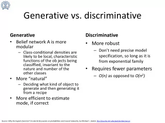
HMM-based adaptation and discriminative training are important techniques for improving accuracy Both procedures start with HMM’s ML parameters ◮ Estimated using a large training corpus drawn from many speakers Both procedures adjust the model parameters ◮ Adaptation: model estimation using limited, novel data ◮ Discriminative training: uses “discriminative” estimation criteria However the goals of the two procedures differ: ◮ Adaptation: specialization ◮ Discriminative training: compensation for model failures

What is acoustic model adaptation? A procedure to adapt or target a speech recognizer to ◮ A specific acoustic environment ◮ A particular speaker To understand how this works, we need to understand ◮ The adaptation problem ◮ Two adaptation procedures

HMM parameters We use (mixtures of) multivariate normal distributions for our output distributions For simplicity we will discuss 1-dimensional, unimodal models, so the distribution for state l (there are L ≡ L ( M ) states) i . i . d ∼ N ( µ l , σ 2 x | q l l ) Thus the parameters of our acoustic models consist of ◮ means and variances for the output distributions (important) ◮ the transition matrices for the states (not so important for speech recognition)

We use HMMs to model triphones A triphone is just a phone in context ◮ Phone b preceded by a, followed by c: a-b+c We typically use three state HMMs for each triphone There is tremendous variability in the amount of training data for each triphone ◮ We cluster triphones (at the state level) ◮ Top-down clustering using decision trees

The acoustic model adaptation problem We have generic models trained/estimated from a large amount of data recorded from many speakers ◮ Usually we train from thousands of hours of recordings from thousands of speakers We are given a relatively small amount of novel data ◮ From a new/unseen acoustic environment (say 20 hours) ◮ From a new speaker (maybe as little as a minute) Our task is to obtain new model parameters that are a better fit for this new task or speaker ◮ We will sacrifice some of the generic model’s generality

The acoustic model adaptation problem (cont’d) We preserve the structure of the generic HMM ◮ We only adjust the output distribution means and variances In particular, we do not retrain starting from scratch with the new data ◮ We do not have enough data to train full blown models Hence the terminology adaptation

We need transcripts for training w 1 w 2 w 3 p 1 p 2 s 3 s 4 s 5 s 6 s 1 s 2 o 3 o 4 o 5 o 6 o 1 o 2 c 1 c 1 c 1 c 1 c 1 c 1 c 2 c 2 c 2 c 2 c 2 c 2 ... ... ... ... ... ... c 39 c 39 c 39 c 39 c 39 c 39 Notation: s = q states, o = x observations

Two modes of adaptation Adaptation data is just like training data in that it consists of transcribed audio data ◮ How do we get the transcripts? Supervised adaptation ◮ We are given (accurate) transcripts ◮ Closest to training, most accurate, but may not be realistic Unsupervised adaptation ◮ We need to produce the (errorful) transcripts via recognition ◮ Errors in transcripts degrade adaptation performance

The acoustic model adaptation problem (cont’d) For clarity without effecting generality ◮ We will focus on the speaker adaptation problem ◮ We will work in one feature dimension The original models θ SI are speaker independent ◮ Model parameters { µ SI l , σ SI l } L l =1 ◮ Training frames { y t } M t =1 The adapted models θ SD are speaker dependent ◮ Model parameters { µ SD , σ SD } L l l l =1 ◮ Training frames { x t } N t =1

An idealized view of the training data The oval represents the SI training data with the circles representing the observed training data from the individual training speakers ✬ ✩ ✛✘ ✛✘ ✛✘ ✛✘ ✛✘ ✚✙ ✚✙ ✚✙ ✚✙ ✚✙ ✛✘ ✛✘ ✛✘ ✛✘ ✛✘ ✚✙ ✚✙ ✚✙ ✚✙ ✚✙ ✛✘ ✛✘ ✛✘ ✛✘ ✛✘ ✚✙ ✚✙ ✚✙ ✚✙ ✚✙ ✫ ✪

An idealized view of the adaptation problem The circle outside of the oval represents all of the data ever produced by the new target speaker, while the black disk is the data we observe ( { x t } N t =1 ) ✬ ✩ ✛✘ ✛✘ ✛✘ ✛✘ ✛✘ ✚✙ ✚✙ ✚✙ ✚✙ ✚✙ ✛✘ ✛✘ ✛✘ ✛✘ ✛✘ ✛✘ ✉ ✚✙ ✚✙ ✚✙ ✚✙ ✚✙ ✚✙ ✛✘ ✛✘ ✛✘ ✛✘ ✛✘ ✚✙ ✚✙ ✚✙ ✚✙ ✚✙ ✫ ✪

The adaptation problem restated To adjust the generic speaker independent model so it becomes specialized to the target speaker Given the small sample from the target speaker ( { x t } N t =1 ) we estimate speaker dependent means for all of the states that ◮ Fit/explain the small sample that we’ve been given ◮ Fit/explain all future data generated by this speaker We will use statistical inference ◮ We also want to leverage the prior knowledge that the generic models summarize

The speaker independent means A key part of the Baum-Welch algorithm for HMM parameter estimation is determining the probability distribution of the hidden states across a given frame y t : ◮ p ( q t l | y , θ SI ) ◮ � L l =1 p ( q t l | y , θ SI ) = 1 ◮ p ( q t l | y , θ SI ) is the fraction of frame y t that is assigned to state q l (at time t ) Then the ML estimate of the speaker independent mean for state l is the average of the fractional frames assigned to l : � M t =1 p ( q t l | y , θ SI ) y t µ SI ˆ = l � M t =1 p ( q t l | y , θ SI )

A naive approach to adaptation We use θ SI to compute the fractional counts and set � N t =1 p ( q t l | x , θ SI ) x t µ SD ˆ = l � N t =1 p ( q t l | x , θ SI ) It’s useful to introduce the total of the estimated fractional count of frames assigned to state l : N n SD � p ( q t l | x , θ SI ) ˆ ≡ l t =1 Where L � n SD ˆ = N l l =1

Problems with the naive approach: uneven counts n SD The distribution of the adaptation data across the states (ˆ ) l will be far from uniform ◮ Some states, notably silence, will have a large fraction of the n SD data (ˆ / N ) l ◮ Other states will not have any adaptation data, i.e. ˆ n SD = 0 l ◮ This will be exacerbated when N is small µ SD The resulting estimates, ˆ , will vary in reliability l ◮ If ˆ n SD µ SD > 50, then ˆ is probably a pretty good estimate l l ◮ If ˆ n SD µ SD < 4, then ˆ is probably not a very good estimate l l n SD µ SD ◮ If ˆ = 0, then ˆ doesn’t even make sense l l

Problems with the naive approach: unreliable counts Suppose the speaker dependent data is very different from the speaker independent models (or training data) ◮ Heavy accent ◮ Novel channel This can result in unreliable fractional counts which are inputs µ SD to the estimates ˆ l ◮ p ( q t l | x , θ SI ) Unsupervised adaptation also leads to unreliable counts

Another naive approach: add { x t } N t =1 to the training data If we simply add the speakers data { x t } N t =1 to the training data { x t } N t =1 and re-estimate, then the resulting means are n SI µ SI n SD µ SD = ˆ l ˆ + ˆ ˆ µ ML l l l ˆ l n SI n SD ˆ + ˆ l l n SI n SD Since we are assuming ˆ >> ˆ we will have l l µ ML µ SI ˆ ≈ ˆ l l Related question: when do we have enough data to directly estimate SD models?

Two linear adaptation methods Two linear methods have been developed to address the problem of uneven counts ◮ MAP (maximum a posteriori ) ◮ MLLR (maximum likelihood linear regression) Multiple adaptation passes address the problem of unreliable counts MAP and MLLR are examples of empirical Bayes estimation

Empirical Bayes (Robbins 1951, Efron and Morris 1973) In traditional Bayesian analysis prior distributions are chosen before any data are observed ◮ In empirical Bayes prior distributions are estimated from the data A example from baseball (Efron-Morris) ◮ We know the batting averages of 18 players after their first 45 at bats ( { x i } 18 i =1 ) ◮ We want to predict their batting averages at the end of the season (after 450 at bats) The obvious solution is to use the early season averages individually ◮ We predict that player i will have average x i

Empirical Bayes (cont’d) There is a better solution that takes into account all of the available information: y i = ¯ x + c ( x i − ¯ x ) ◮ ¯ x is the average of the x i ◮ c is a “shrinkage factor” compute from the x i (related to the variance) ◮ 0 < c < 1 ◮ ¯ x and c are empirical estimates of the prior distribution of the observed x i .

Empirical Bayes applies to adaptation problem Our adaptation problem is very similar to the baseball problem ◮ However, we are going to leverage more prior information ◮ Analogous to prior seasons information with other players MAP and MLLR use the same empirical prior: ◮ The estimates from the training data { ˆ µ SI σ SI l } L l , ˆ l =1 This empirical prior is used to adjust the speaker dependent µ SD } L means, { ˆ l =1 , to obtain new estimates: l ◮ MAP uses interpolation ◮ MLLR uses weighted least squares