History matching real production and seismic data for the Norne - PowerPoint PPT Presentation
History matching real production and seismic data for the Norne field EnKF Workshop 2018 Rolf J. Lorentzen, Tuhin Bhakta, Dario Grana, Xiaodong Luo, Randi Valestrand, Geir Nvdal, Ivar Sand Introduction The full norne model is history
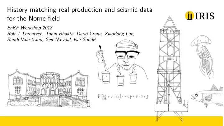
History matching real production and seismic data for the Norne field EnKF Workshop 2018 Rolf J. Lorentzen, Tuhin Bhakta, Dario Grana, Xiaodong Luo, Randi Valestrand, Geir Nævdal, Ivar Sandø
Introduction • The full norne model is history matched using real production and seismic data • Initial ensemble generated using Gaussian random fields • Updates PORO, PERMX, NTG, MULTZ, MULTFLT, MULTREGT, KRW/KRG, OWC • Clay content defined as VCLAY = 1 - NTG • Sequential assimilation (production → seismic) • Seismic data inverted for acoustic impedance at four points in time • Iterative ensemble smoother, RLM-MAC, used (Luo et. al, SPE-176023-PA) • Sparse representation using wavelets (data reduced by 86 %) • Correlation based localization
Seismic data inversion and transformation • Time shift correction: Alfonzo et al. 2017 • Linearized Bayesian approach: Buland and Omre, 2003: S base = Gy base + e • Time to depth conversion: Provided Norne velocity model • Upscaling: Petrel software • Difference and averaging: o ∆ z p
Petro-elastic model • Estimate mineral bulk and shear moduli: [ K s , G s ] ← Hashin − Shtrikman ( K quartz , G quartz , K clay , G clay , V clay ) • Dry rock bulk and shear moduli (empirical): [ K dry , G dry ] ← f ( p , p ini , φ ) • Fluid substitution: [ K sat , G sat ] ← Gassman ( K dry , G dry , K s , G s ) • P-wave velocity and rock density: [ v p , ρ sat ] ← Mavko ( K sat , G sat ) z p = v p × ρ sat
Sparse representation and image denoising 1. Transform seismic observations: o HLH c S ← DWT (∆ z p ) HHH LLH LHH HHL LLL LHL
Sparse representation and image denoising 1. Transform seismic observations: o HLH c S ← DWT (∆ z p ) 2. Estimate noise in each subband (MAD): σ S = median ( | c S − median ( c S ) | ) / 0 . 6745 HHH LLH LHH HHL LLL LHL
Sparse representation and image denoising 1. Transform seismic observations: o HLH c S ← DWT (∆ z p ) 2. Estimate noise in each subband (MAD): σ S = median ( | c S − median ( c S ) | ) / 0 . 6745 HHH LLH LHH 3. Compute standard deviation for coefficients: σ S = std ( c S ) ˆ HHL LLL LHL
Sparse representation and image denoising 1. Transform seismic observations: o HLH c S ← DWT (∆ z p ) 2. Estimate noise in each subband (MAD): σ S = median ( | c S − median ( c S ) | ) / 0 . 6745 HHH LLH LHH 3. Compute standard deviation for coefficients: σ S = std ( c S ) ˆ HHL LLL LHL 4. Compute truncation value (Bayesian shrinkage): σ 2 √ T S = S | σ 2 σ 2 S − ˆ S |
Sparse representation and image denoising 1. Transform seismic observations: o HLH c S ← DWT (∆ z p ) 2. Estimate noise in each subband (MAD): σ S = median ( | c S − median ( c S ) | ) / 0 . 6745 HHH LLH LHH 3. Compute standard deviation for coefficients: σ S = std ( c S ) ˆ HHL LLL LHL 4. Compute truncation value (Bayesian shrinkage): σ 2 √ T S = S | σ 2 σ 2 S − ˆ S | 5. Apply hard thresholding: d o = c ( I ) c s → c s > T S ,
Ensemble smoother d ) T + γ i C d ] − 1 × [ d o + ǫ j − d i m i +1 = m i j + S i m ( S i d ) T [ S i d ( S i j ] j ↓ TSVD j + ˜ K i ∆˜ m i +1 = m i d i j j ∆˜ j ∈ R p × 1 , p ≤ N : Projected (“effective”) data innovation. d i
Correlation based localization 1. Compute sample correlation between parameters ( k ) and “effective” measurements ( l ): ρ kl ∈ R N m × p
Correlation based localization 1. Compute sample correlation between parameters ( k ) and “effective” measurements ( l ): ρ kl ∈ R N m × p 2. Transform all correlations for each observation ( ρ l ), and return high-frequency coefficients: c H ← DWT ( ρ l ) l
Correlation based localization 1. Compute sample correlation between parameters ( k ) and “effective” measurements ( l ): ρ kl ∈ R N m × p 2. Transform all correlations for each observation ( ρ l ), and return high-frequency coefficients: c H ← DWT ( ρ l ) l 3. Estimate noise in coefficients (MAD): σ l = median ( | c H l − median ( c H l ) | ) / 0 . 6745
Correlation based localization 1. Compute sample correlation between parameters ( k ) and “effective” measurements ( l ): ρ kl ∈ R N m × p 2. Transform all correlations for each observation ( ρ l ), and return high-frequency coefficients: c H ← DWT ( ρ l ) l 3. Estimate noise in coefficients (MAD): σ l = median ( | c H l − median ( c H l ) | ) / 0 . 6745 4. Compute truncation value (universal rule): � λ l = max( 2 ln n ( ρ l ) σ l )
Correlation based localization 1. Compute sample correlation between parameters ( k ) and “effective” measurements ( l ): ρ kl ∈ R N m × p 2. Transform all correlations for each observation ( ρ l ), and return high-frequency coefficients: c H ← DWT ( ρ l ) l 3. Estimate noise in coefficients (MAD): σ l = median ( | c H l − median ( c H l ) | ) / 0 . 6745 4. Compute truncation value (universal rule): � λ l = max( 2 ln n ( ρ l ) σ l ) 5. Compute truncation matrix: ξ kl = 1 , if | ρ kl | ≥ λ l , 0 otherwise
Correlation based localization 1. Compute sample correlation between parameters ( k ) and “effective” measurements ( l ): ρ kl ∈ R N m × p 2. Transform all correlations for each observation ( ρ l ), and return high-frequency coefficients: c H ← DWT ( ρ l ) l 3. Estimate noise in coefficients (MAD): σ l = median ( | c H l − median ( c H l ) | ) / 0 . 6745 4. Compute truncation value (universal rule): � λ l = max( 2 ln n ( ρ l ) σ l ) 5. Compute truncation matrix: ξ kl = 1 , if | ρ kl | ≥ λ l , 0 otherwise 6. Updated Kalman gain matrix (see also Luo and Bhakta, 2017): K = ξ ◦ ˜ ˆ K
Measurement operator The observation operator G comprises several steps summarized as: 1. running the reservoir simulator using m j to compute dynamic variables (pressure and saturation)
Measurement operator The observation operator G comprises several steps summarized as: 1. running the reservoir simulator using m j to compute dynamic variables (pressure and saturation) 2. running the PEM to compute the acoustic impedance, z p , j , at all survey times
Measurement operator The observation operator G comprises several steps summarized as: 1. running the reservoir simulator using m j to compute dynamic variables (pressure and saturation) 2. running the PEM to compute the acoustic impedance, z p , j , at all survey times 3. compute differences and average over formation layers to get ∆ z p , j
Measurement operator The observation operator G comprises several steps summarized as: 1. running the reservoir simulator using m j to compute dynamic variables (pressure and saturation) 2. running the PEM to compute the acoustic impedance, z p , j , at all survey times 3. compute differences and average over formation layers to get ∆ z p , j 4. applying the DWT to get c j
Measurement operator The observation operator G comprises several steps summarized as: 1. running the reservoir simulator using m j to compute dynamic variables (pressure and saturation) 2. running the PEM to compute the acoustic impedance, z p , j , at all survey times 3. compute differences and average over formation layers to get ∆ z p , j 4. applying the DWT to get c j 5. using the leading indices I to get d j = c j ( I )
Generate initial ensemble Compute Assimilate wavelet coeff. production data c o = DWT (∆ z o p ) Compute data Find indices for d j = G ( m j ), leading coeff. ( I ) j = 1 . . . N Iterate Compute noise Compute tapering ( C d ) and data matrix ξ corr d o = c o ( I ) Update parame- ters m 1 , . . . , m N Figure: Workflow for assimilating seismic data.
Norne field • Grid size: 46 x 112 x 22 (113344) • Active cells: 44927 • Wells: 9 injectors, 27 producers • Production: 3312 days
Initial Production Seismic
Initial Production Seismic
Initial Production Seismic
Initial Production Seismic
Top: real data. Middle: production. Bottom: seismic.
Initial Production Seismic
Initial Production Seismic
Initial Production Seismic
Summary / Conclusions • A workflow for history matching real production and seismic data is presented • Clay content and other petrophysical parameters updated • Data match improved for both production and seismic data • Updated static fields are geologically credible • Potential for simulating infill wells or EOR strategies
Acknowledgments We thank • Schlumberger and CGG for providing academic software licenses to ECLIPSE and HampsonRussell, respectively. • Main financial support from Eni, Petrobras, and Total, as well as the Research Council of Norway (PETROMAKS2). • Partial financial support from The National IOR Centre of Norway.
Recommend
More recommend
Explore More Topics
Stay informed with curated content and fresh updates.
