High performance mantle convection modeling Jens Weism uller, Bj - PowerPoint PPT Presentation
Introduction Equations HPC methods Asthenosphere Conclusions High performance mantle convection modeling Jens Weism uller, Bj orn Gmeiner, Siavash Ghelichkhan, Markus Huber, Lorenz John, Barbara Wohlmuth, Ulrich R ude and Hans-Peter
Introduction Equations HPC methods Asthenosphere Conclusions High performance mantle convection modeling Jens Weism¨ uller, Bj¨ orn Gmeiner, Siavash Ghelichkhan, Markus Huber, Lorenz John, Barbara Wohlmuth, Ulrich R¨ ude and Hans-Peter Bunge Geophysics Department of Earth- and Environmental Sciences Ludwig-Maximilians-Universit¨ at M¨ unchen SPPEXA annual plenary meeting, 25.01.2016 T ERRA Weism¨ uller et al. High performance mantle convection modeling 1/26
Introduction Equations HPC methods Asthenosphere Conclusions The Earth’s mantle • Solid layer between crust and core • Makes up about 84% of the Earth’s volume • Solid, but ductile • Creeping, viscous flow • Convects on time scales of cm/a Image: mail.colonial.net Weism¨ uller et al. High performance mantle convection modeling 2/26
Introduction Equations HPC methods Asthenosphere Conclusions Mantle Convection • Regulates the long term thermal evolution of the Earth • Controls heat loss of the core • Driving force behind plate tectonics Image: mail.colonial.net Weism¨ uller et al. High performance mantle convection modeling 3/26
Introduction Equations HPC methods Asthenosphere Conclusions Plate tectonics • Earth’s magnetic field alternates polarity Image: geology.sdsu.edu • Solidifying rock takes on the current magnetic field of the Earth • Residual magnetization can be used to reconstruct tectonic plate motion history Weism¨ uller et al. High performance mantle convection modeling 4/26
Introduction Equations HPC methods Asthenosphere Conclusions Seismic tomography • Seismic tomography images shear velocities in the mantle • Using mineralogic models, they can be converted to buoyancies Ritsema et al, S40RTS Weism¨ uller et al. High performance mantle convection modeling 5/26
Introduction Equations HPC methods Asthenosphere Conclusions Seismic tomography • Seismic tomography images shear velocities in the mantle • Using mineralogic models, they can be converted to buoyancies Together with plate velocities: Terminal and boundary conditions Weism¨ uller et al. High performance mantle convection modeling 6/26
Introduction Equations HPC methods Asthenosphere Conclusions Brief history of mantle Glatzmeier, 1988 Baumgardner, 1985 convection modeling • Global models became available in the late 80s • They were parallelized in the 90s Bunge and Baumgardner, 1995 Tackley et al, 1993 Weism¨ uller et al. High performance mantle convection modeling 7/26
Introduction Equations HPC methods Asthenosphere Conclusions Zhong et al, 2007 • Convective planform (Earth and other planets) • Link to seismology • Geodetic observations • Mineralogy • Rheological effects • Thermal evolution • . . . Schuberth et al, 2009 Tackley, 2012 Weism¨ uller et al. High performance mantle convection modeling 8/26
Introduction Equations HPC methods Asthenosphere Conclusions Towards extreme resolutions • Most classic codes scale to ∼ 1 , 000 processors • Current supercomputers have ∼ 1 , 000 , 000 cores • New class of problems: ◮ Fluid dynamic inverse models ◮ Complex non-linear problems Weism¨ uller et al. High performance mantle convection modeling 9/26
Introduction Equations HPC methods Asthenosphere Conclusions Future applications: Adjoint • Reconstruct past state of the mantle with inverse models • Start from initial guess • Iteratively run forward and backwards simulations Ghelichkhan et al, submitted Weism¨ uller et al. High performance mantle convection modeling 10/26
Introduction Equations HPC methods Asthenosphere Conclusions Complex, non-linear rheologies Deformation mechanisms of MgO: • Classically, flow laws are linear: η = f ( x , T ) • Non-linear behaviour increasingly in focus: η = f ( x , T , v ) • Conventional stress-strain-relations might not hold: η =? Cordier et al, 2012 ⇒ Will need to deal with computationally challenging rheologies Weism¨ uller et al. High performance mantle convection modeling 11/26
Introduction Equations HPC methods Asthenosphere Conclusions Governing equations � η ∆ u − ∇ p + Ra T = 0 Stokes equations ∇ · u = 0 ∂ t T = − u · ∇ T − κ ∆ T } Heat equation • Simplified Navier-Stokes equations • Slow deformation by creep Weism¨ uller et al. High performance mantle convection modeling 12/26
Introduction Equations HPC methods Asthenosphere Conclusions Governing equations � η ∆ u − ∇ p + Ra T = 0 Stokes equations ∇ · u = 0 ∂ t T = − u · ∇ T − κ ∆ T } Heat equation • Simplified Navier-Stokes equations • Slow deformation by creep • Force balance between friction and buoyancy Weism¨ uller et al. High performance mantle convection modeling 12/26
Introduction Equations HPC methods Asthenosphere Conclusions Governing equations � η ∆ u − ∇ p + Ra T = 0 Stokes equations ∇ · u = 0 ∂ t T = − u · ∇ T − κ ∆ T } Heat equation • Simplified Navier-Stokes equations • Slow deformation by creep • Force balance between friction and buoyancy • Dominated by viscous term η ∆ u ⇒ Global models Weism¨ uller et al. High performance mantle convection modeling 12/26
Introduction Equations HPC methods Asthenosphere Conclusions Governing equations � η ∆ u − ∇ p + Ra T = 0 Stokes equations ∇ · u = 0 ∂ t T = − u · ∇ T − κ ∆ T } Heat equation • Simplified Navier-Stokes equations • Slow deformation by creep • Force balance between friction and buoyancy • Dominated by viscous term η ∆ u ⇒ Global models • Time derivative only in heat equation Weism¨ uller et al. High performance mantle convection modeling 12/26
Introduction Equations HPC methods Asthenosphere Conclusions Governing equations � η ∆ u − ∇ p + Ra T = 0 Stokes equations ∇ · u = 0 ∂ t T = − u · ∇ T − κ ∆ T } Heat equation Start with initial T Solve Stokes equations for u and p Integrate heat equation for T forward in time Weism¨ uller et al. High performance mantle convection modeling 13/26
Introduction Equations HPC methods Asthenosphere Conclusions Governing equations � η ∆ u − ∇ p + Ra T = 0 Stokes equations ∇ · u = 0 ∂ t T = − u · ∇ T − κ ∆ T } Heat equation Start with initial T Solve Stokes equations for u and p Integrate heat equation for T forward in time Weism¨ uller et al. High performance mantle convection modeling 13/26
Introduction Equations HPC methods Asthenosphere Conclusions Solving the Stokes equations � η ∆ u − ∇ p + Ra T = 0 Stokes equations ∇ · u = 0 ∂ t T = − u · ∇ T − κ ∆ T } Heat equation • So called saddle point problem: � A � � u � f � � B T = B 0 p 0 • Many possible solution schemes • Expensive part is solution of Au = f Weism¨ uller et al. High performance mantle convection modeling 14/26
Introduction Equations HPC methods Asthenosphere Conclusions Adaptive mesh refinement • Flow structures evolve down to the kilometer-scale • Refine the mesh where things happen • Administrational overhead Burstedde et al, 2013 Kronbichler et al, 2012 Weism¨ uller et al. High performance mantle convection modeling 15/26
Introduction Equations HPC methods Asthenosphere Conclusions Extreme resolutions Alternative Concept: • Equal resolution throughout the mantle + No administrative overhead – Computational overhead in areas that need no high resolution Weism¨ uller et al. High performance mantle convection modeling 16/26
Introduction Equations HPC methods Asthenosphere Conclusions Hierarchical Hybrid Grids • Discretizing a planet not possible with fully structured grid • More efficient solvers on structured grids Block-structured grid: • Unstructured input mesh as multigrid’s coarse grid • Regularly refined Weism¨ uller et al. High performance mantle convection modeling 17/26
Introduction Equations HPC methods Asthenosphere Conclusions Hierarchical Hybrid Grids On input mesh: Geometric hierarchy of ... • Volumes (tetrahedra) • Faces (triangles) • Edges • Nodes Communication reduction by • Independent solution within geometric elements • Communication of ghost layers Weism¨ uller et al. High performance mantle convection modeling 18/26
Introduction Equations HPC methods Asthenosphere Conclusions Hierarchical Hybrid Grids Matrix free stencil code • Fully stencil-based for constant viscosity (30 FLOPS per grid point and operator evaluation) • Efficient on-the-fly stencil assembly for more complex cases Weism¨ uller et al. High performance mantle convection modeling 19/26
Introduction Equations HPC methods Asthenosphere Conclusions The asthenosphere • Mechanically weak uppermost layer of the mantle • Traditionally: plausible depth extent of 660 km • Low viscosity: 10 18 − 10 20 Pa s (compared to ≈ 10 22 Pa s in the lower mantle) • Possible causes: Partial melting, water, mineralogy (p/T) Weism¨ uller et al. High performance mantle convection modeling 20/26
Introduction Equations HPC methods Asthenosphere Conclusions Thickness of the asthenosphere from seismology • Full waveform seismic tomography studies have imaged a thin horizontal layer of 100 − 200 km depth extent Fichtner, 2009 Weism¨ uller et al. High performance mantle convection modeling 21/26
Recommend
More recommend
Explore More Topics
Stay informed with curated content and fresh updates.

