Hierarchy An arrangement or classification of things according to - PowerPoint PPT Presentation
Hierarchy An arrangement or classification of things according to inclusiveness A natural way of abstraction, summarization, compression, and simplification for understanding Typical setting: organize a given set of objects to a
Hierarchy • An arrangement or classification of things according to inclusiveness • A natural way of abstraction, summarization, compression, and simplification for understanding • Typical setting: organize a given set of objects to a hierarchy – No or very little supervision – Some heuristic quality guidances on the quality of the hierarchy Jian Pei: CMPT 459/741 Clustering (2) 1
Hierarchical Clustering • Group data objects into a tree of clusters • Top-down versus bottom-up Step 3 Step 4 Step 1 Step 2 Step 0 agglomerative (AGNES) a a b b a b c d e c c d e d d e e divisive Step 1 Step 0 (DIANA) Step 3 Step 2 Step 4 Jian Pei: CMPT 459/741 Clustering (2) 2
AGNES (Agglomerative Nesting) • Initially, each object is a cluster • Step-by-step cluster merging, until all objects form a cluster – Single-link approach – Each cluster is represented by all of the objects in the cluster – The similarity between two clusters is measured by the similarity of the closest pair of data points belonging to different clusters Jian Pei: CMPT 459/741 Clustering (2) 3
Dendrogram • Show how to merge clusters hierarchically • Decompose data objects into a multi- level nested partitioning (a tree of clusters) • A clustering of the data objects: cutting the dendrogram at the desired level – Each connected component forms a cluster Jian Pei: CMPT 459/741 Clustering (2) 4
DIANA (Divisive ANAlysis) • Initially, all objects are in one cluster • Step-by-step splitting clusters until each cluster contains only one object 10 10 10 9 9 9 8 8 8 7 7 7 6 6 6 5 5 5 4 4 4 3 3 3 2 2 2 1 1 1 0 0 0 0 1 2 3 4 5 6 7 8 9 10 0 1 2 3 4 5 6 7 8 9 10 0 1 2 3 4 5 6 7 8 9 10 Jian Pei: CMPT 459/741 Clustering (2) 5
Distance Measures d ( C , C ) min d ( p , q ) • Minimum distance = min i j p C , q C ∈ ∈ i j • Maximum distance d ( C , C ) max d ( p , q ) = max i j p C , q C ∈ ∈ i j • Mean distance d ( C , C ) d ( m , m ) = mean i j i j • Average distance 1 d ( C , C ) d ( p , q ) ∑ ∑ = avg i j n n p C q C i j ∈ ∈ i j m: mean for a cluster C: a cluster n: the number of objects in a cluster Jian Pei: CMPT 459/741 Clustering (2) 6
Challenges • Hard to choose merge/split points – Never undo merging/splitting – Merging/splitting decisions are critical • High complexity O(n 2 ) • Integrating hierarchical clustering with other techniques – BIRCH, CURE, CHAMELEON, ROCK Jian Pei: CMPT 459/741 Clustering (2) 7
BIRCH • Balanced Iterative Reducing and Clustering using Hierarchies • CF (Clustering Feature) tree: a hierarchical data structure summarizing object info – Clustering objects à clustering leaf nodes of the CF tree Jian Pei: CMPT 459/741 Clustering (2) 8
Clustering Feature Vector Clustering Feature: CF = (N, LS, SS) N : Number of data points LS: ∑ N i=1 =o i CF = (5, (16,30),(54,190)) SS: ∑ N i=1 =o i 2 (3,4) 10 9 (2,6) 8 7 6 (4,5) 5 4 3 (4,7) 2 1 (3,8) 0 0 1 2 3 4 5 6 7 8 9 10 Jian Pei: CMPT 459/741 Clustering (2) 9
CF-tree in BIRCH • Clustering feature: – Summarize the statistics for a cluster – Many cluster quality measures (e.g., radium, distance) can be derived – Additivity: CF 1 +CF 2 =(N 1 +N 2 , L 1 +L 2 , SS 1 +SS 2 ) • A CF tree: a height-balanced tree storing the clustering features for a hierarchical clustering – A nonleaf node in a tree has descendants or “children” – The nonleaf nodes store sums of the CFs of children Jian Pei: CMPT 459/741 Clustering (2) 10
CF Tree B = 7 CF 1 CF 2 CF 3 CF 6 Root L = 6 child 1 child 2 child 3 child 6 Non-leaf node CF 1 CF 2 CF 3 CF 5 child 1 child 2 child 3 child 5 Leaf node Leaf node prev CF 1 CF 2 CF 6 next prev CF 1 CF 2 CF 4 next Jian Pei: CMPT 459/741 Clustering (2) 11
Parameters of a CF-tree • Branching factor: the maximum number of children • Threshold: max diameter of sub-clusters stored at the leaf nodes Jian Pei: CMPT 459/741 Clustering (2) 12
BIRCH Clustering • Phase 1: scan DB to build an initial in- memory CF tree (a multi-level compression of the data that tries to preserve the inherent clustering structure of the data) • Phase 2: use an arbitrary clustering algorithm to cluster the leaf nodes of the CF-tree Jian Pei: CMPT 459/741 Clustering (2) 13
Pros & Cons of BIRCH • Linear scalability – Good clustering with a single scan – Quality can be further improved by a few additional scans • Can handle only numeric data • Sensitive to the order of the data records Jian Pei: CMPT 459/741 Clustering (2) 14
Drawbacks of Square Error Based Methods • One representative per cluster – Good only for convex shaped having similar size and density • K: the parameter of number of clusters – Good only if k can be reasonably estimated Jian Pei: CMPT 459/741 Clustering (2) 15
CURE: the Ideas • Each cluster has c representatives – Choose c well scattered points in the cluster – Shrink them towards the mean of the cluster by a fraction of α – The representatives capture the physical shape and geometry of the cluster • Merge the closest two clusters – Distance of two clusters: the distance between the two closest representatives Jian Pei: CMPT 459/741 Clustering (2) 16
Cure: The Algorithm • Draw random sample S • Partition sample to p partitions • Partially cluster each partition • Eliminate outliers – Random sampling + remove clusters growing too slowly • Cluster partial clusters until only k clusters left – Shrink representatives of clusters towards the cluster center Jian Pei: CMPT 459/741 Clustering (2) 17
Data Partitioning and Clustering y y y x x x y y x x Jian Pei: CMPT 459/741 Clustering (2) 18
Shrinking Representative Points • Shrink the multiple representative points towards the gravity center by a fraction of α • Representatives capture the shape y y è x x Jian Pei: CMPT 459/741 Clustering (2) 19
Clustering Categorical Data: ROCK • Robust Clustering using links – # of common neighbors between two points – Use links to measure similarity/proximity – Not distance based O n ( 2 nm m n 2 log ) n – + + m a • Basic ideas: T T ∩ – Similarity function and neighbors: Sim T T ( , ) 1 2 = 1 2 T T ∪ 1 2 • Let T1 = {1,2,3}, T2={3,4,5} { } 3 1 Sim T ( 1 , T 2 ) 0 2 . = = = { , , , , } 1 2 3 4 5 5 Jian Pei: CMPT 459/741 Clustering (2) 20
Limitations • Merging decision based on static modeling – No special characteristics of clusters are considered C1 C2 C1 ’ C2 ’ CURE and BIRCH merge C1 and C2 C1 ’ and C2 ’ are more appropriate for merging Jian Pei: CMPT 459/741 Clustering (2) 21
Chameleon • Hierarchical clustering using dynamic modeling • Measures the similarity based on a dynamic model – Interconnectivity & closeness (proximity) between two clusters vs interconnectivity of the clusters and closeness of items within the clusters • A two-phase algorithm – Use a graph partitioning algorithm: cluster objects into a large number of relatively small sub-clusters – Find the genuine clusters by repeatedly combining sub- clusters Jian Pei: CMPT 459/741 Clustering (2) 22
Overall Framework of CHAMELEON Construct Sparse Graph Partition the Graph Data Set Merge Partition Final Clusters Jian Pei: CMPT 459/741 Clustering (2) 23
To-Do List • Read Chapter 10.3 • (for thesis-based graduate students only) read the paper “BIRCH: an efficient data clustering method for very large databases” Jian Pei: CMPT 459/741 Clustering (2) 24
Recommend
More recommend
Explore More Topics
Stay informed with curated content and fresh updates.

