Hi Matlab Grader homework, emailed Thursday, 1 (of 9) homeworks Due - PowerPoint PPT Presentation

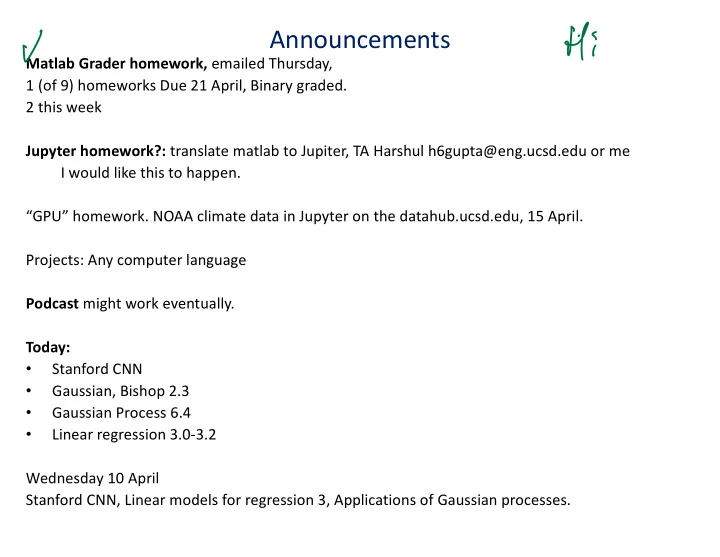
Announcements Hi Matlab Grader homework, emailed Thursday, 1 (of 9) homeworks Due 21 April, Binary graded. 2 this week Jupyter homework?: translate matlab to Jupiter, TA Harshul h6gupta@eng.ucsd.edu or me I would like this to happen. “GPU” homework. NOAA climate data in Jupyter on the datahub.ucsd.edu, 15 April. Projects: Any computer language Podcast might work eventually. Today: Stanford CNN • • Gaussian, Bishop 2.3 Gaussian Process 6.4 • Linear regression 3.0-3.2 • Wednesday 10 April Stanford CNN, Linear models for regression 3, Applications of Gaussian processes.

Bayes and Softmax (Bishop p. 198) Bayes: • Parametric Approach: Linear Classifier 3072x1 O p ( x | y ) = p ( y | x ) p ( x ) p ( y | x ) p ( x ) f(x,W) = Wx + b 10x1 = Image p ( y ) P y ∈ Y p ( x, y ) 10x1 10x3072 10 numbers giving f( x , W ) class scores Classification of N classes: • it C Array of 32x32x3 numbers W (3072 numbers total) parameters p ( x |C n ) p ( C n ) or weights p ( C n | x ) = Fei-Fei Li & Justin Johnson & Serena Yeung Lecture 2 - 54 April 6, 2017 P N k =1 p ( x |C k ) p ( C k ) exp( a n ) = So P N k =1 exp( a k ) with Et a n = ln ( p ( x |C n ) p ( C n ))

Softmax to Logistic Regression (Bishop p. 198) p ( x |C 1 ) p ( C 1 ) p ( C 1 | x ) = P 2 k =1 p ( x |C k ) p ( C k ) exp( a 1 ) 1 = = P 2 1 + exp( − a ) k =1 exp( a k ) with a = ln p ( x |C 1 ) p ( C 1 ) p ( x |C 2 ) p ( C 2 ) s for binary classification we should use logis

Softmax with Gaussian(Bishop p. 198) C p ( x |C n ) p ( C n ) p ( C n | x ) = P N k =1 p ( x |C k ) p ( C k ) exp( a n ) I = xc NLM.is P N k =1 exp( a k ) with a n = ln ( p ( x |C n ) p ( C n )) |C C EH ANTE'aripen 2 e Assuming x is Gaussian N ( µ n , Σ ) orm, it can be shown that (7) can be ex cncpfxknj EVTEIEMTE.fi a n = w T n x + w 0 mish w n = Σ − 1 µ n w w 0 = − 1 w 2 µ T n Σ − 1 µ n + ln( p ( C n )) n Wo Wii EMTs qxqq two X 87 0 tea Had we

Entropy 1.6 Important quantity in • coding theory • statistical physics • machine learning

The Kullback-Leibler Divergence P true distribution, q is approximating distribution a distance meals are not

KL homework Support of P and Q = > “only >0” don’t use isnan isinf • • After you pass. Take your time to clean up. Get close to 50

Lecture 3 Homework • Pod-cast lecture on-line • • Next lectures: – I posted a rough plan. – It is flexible though so please come with suggestions

Bayes for linear model ! = #$ + & &~N(*, , - ) y ~N(#$, , - ) prior: $~N(*, , $ ) $ 1 = , 1 # 2 , - 34 ! / $ ! ~/ ! $ / $ ~0 $ 1 , , / mean 34 = # 2 , - 34 # + , 5 34 Covariance , 1 IE trig ex xp de ITE't flat y cat µ e e Ax cxtq EE At EAT g µ g e L l xTcf'x XT Cp Xp

Bayes’ Theorem for Gaussian Variables Given • • we have where •

Sequential Estimation of mean (Bishop 2.3.5) Contribution of the N th data point, x N correction given x N correction weight old estimate

Bayesian Inference for the Gaussian (Bishop2.3.6) Assume s 2 is known. Given i.i.d. data the likelihood function for µ is given by UH This has a Gaussian shape as a function of µ (but it is not a distribution over µ ). •

Bayesian Inference for the Gaussian (Bishop2.3.6) Combined with a Gaussian prior over µ , • so this gives the posterior • I T e µ Mart NENG Ast K Mo Iz 2 ENZ

Bayesian Inference for the Gaussian (3) Example: for N = 0, 1, 2 and 10. • Prior

Bayesian Inference for the Gaussian (4) Sequential Estimation 7 I The posterior obtained after observing N-1 data points becomes the prior when we observe the N th data point. Conjugate prior: posterior and prior are in the same family. The prior is called a conjugate prior for the likelihood function.

Gaussian Process (Bishop 6.4, Murphy15) t n = y n + ϵ n I a i O o C ee r l

Gaussian Process (Murphy ch15) T Tz Training n MI K T Kxx

Gaussian Process (Murphy ch15) The conditional is Gaussian: g Common kernel is the squared exponential, RBF, Gaussian kernel r