heaps and heapsort on n elements height of a heap is in (log n ) - PowerPoint PPT Presentation
heaps and heapsort on n elements height of a heap is in (log n ) building a heap bottum-up in O ( n ) analysis via picture (learn) or using summations (know result) data structures and algorithms building a heap one-by-one in O ( n log n ) 2020
heaps and heapsort on n elements height of a heap is in Θ(log n ) building a heap bottum-up in O ( n ) analysis via picture (learn) or using summations (know result) data structures and algorithms building a heap one-by-one in O ( n log n ) 2020 09 17 lecture 6 maxheapify in O (log n ) (also Θ(log n )) heapsort in O ( n log n ); also in Θ( n log n )? yes, see worst-case input or see lower-bound more: see smooth sort use of priority queue: Dijkstra’s algorithm quicksort on n elements input: directed graph G = ( V , E ) with positive weights w and start vertex s in G worst-case in Θ( n 2 ) Algorithm Dijkstra( G , w , s ): initialize( G , s ) best-case in Θ( n log n ) S := ∅ balanced-case in O ( n log n ) Q := G . V while Q � = ∅ do average case (assuming all n ! possible inputs are equally likely) in O ( n log n ) u := extractMin( Q ) expected case (using randomization) in O ( n log n ) S := S ∪ { u } for each v ∈ G . Adj [ u ] do more: replace small recursive calls by insertion sort and sorting networks relax( u , v , w ) the set S contains vertices for which the weight of a shortest path has been found if priority queue implemented with heap then in O ( | E | · log | V | )
overview overview lower bound on sorting lower bound on sorting counting sort counting sort radix sort radix sort bucket sort bucket sort recall: bounds upper and lower bound f , g : N → R + asymptotic upper bound f ∈ O ( g ) asymptotic upper bound: f ( n ) ∈ O ( g ( n )) if f is eventually bound from above by g up to a constant ∃ c > 0 ∈ R + asymptotic tight bound f ∈ Θ( g ) ∃ n 0 > 0 ∈ N f is eventually sandwiched by g up to two constants ∀ n ∈ N : n ≥ n 0 ⇒ f ( n ) ≤ c · g ( n ) asymptotic lower bound f ∈ Ω( g ) asymptotic lower bound: f ( n ) ∈ Ω( g ( n )) if f is eventually bound from below by g up to a constant ∃ c > 0 ∈ R + ∃ n 0 > 0 ∈ N (there are more bounds!) ∀ n ∈ N : n ≥ n 0 ⇒ f ( n ) ≥ c · g ( n )
question lower bound on running time comparison-based sorting: the crucial tests are we consider sorting algorithms based on comparisons k < k ′ a < b , a ≤ b , a = b , a ≥ b , a > b examples: merge sort, heapsort, quicksort which are all decidable in elementary time non-examples: counting sort, bucket sort Ω( n log n ) comparisons are needed in the worst case so far we have seen only comparison-based sorting algorithms so merge sort, heapsort are asymptotically optimal is O ( n log n ) the best worst-case that we have? lowerbound: proof decision tree: example we consider decision trees a < b ? node contains a comparison a < b ? leaf corresponds to a permutation of { 1 , . . . . n } b < c ? b < c ? every comparison-based sorting algorithm has for every number of inputs a decision tree execution of that sorting algorithm corresponds to a path in the tree a < c ? a < c ? c b a a b c every possible permutation (of total n !) must occur a c b b c a c a b b a c every permutation must be reachable
we analyze the height of a decision tree with n nodes we continue to find a bound on the height we have h ≥ ⌈ log n ! ⌉ the number of comparisons is height h of the tree omitting floors and ceilings we find: we have at least n ! (because decision tree), and at most 2 h (because binary tree) leaves, ≥ log( n !) h hence: log(1 · 2 · . . . · ( n 2 − 1) · n = 2 . . . · n ) n ! ≤ #leaves ≤ 2 h log(1 · 1 · . . . · 1 · n 2 . . . · n ≥ 2 ) n ! ≤ 2 h n log(( n 2 ) = 2 ) log n ! ≤ h 2 log( n n = 2 ) h ≥ log n ! hence h ∈ Ω( n log n ) (see also 3.19 in the book that uses Stirling’s approximation) results back to puzzle from Knuth Theorem: any comparison-based sorting algorithm uses Ω( n log n ) comparisons in the worst case. can we sort 5 elements in ⌈ log 5! ⌉ = 7 comparisons? Consequence: heapsort and merge sort are asymptotically optimal However: for specific inputs there are linear sorting algorithms, not based on comparisons
overview counting sort assumption: numbers in input come from fixed range { 0 , . . . , k } . lower bound on sorting algorithm idea: count the number of occurrences of each i from 0 to k counting sort time complexity: in Θ( n + k ) for a input-array of length n radix sort drawback: fixed range, and requires additional counting array C andoutput array B bucket sort counting sort is a stable sorting algorithm what happens if the last loop is done for j := 1 up to j := A . length ? counting sort: pseudo-code overview input array A , output array B , range from 0 up to k Algorithm countingSort( A , B , k ): lower bound on sorting new array C [0 . . . k ] for i := 0 to k do counting sort C [ i ] := 0 radix sort for j := 1 to A . length do C [ A [ j ]] := C [ A [ j ]] + 1 bucket sort for i := 1 to k do C [ i ] := C [ i ] + C [ i − 1] for j := A . length downto 1 do B [ C [ A [ j ]]] := A [ j ] C [ A [ j ]] := C [ A [ j ]] − 1
radix sort radix sort: intuition the old days: used for sorting punched cards 80 columns with one hole in one of the 12 possible places our use: sorting numbers considered as tuples number of columns: (fixed) amout of digits used number of places: 10 for decimal numbers 329 457 329 329 457 657 839 457 657 329 457 657 839 839 657 839 recall the lexicographic ordering for tuples: ( x 1 , . . . , x d ) < ( y 1 , . . . , y d ) if ( x 1 < y 1 ) or (( x 1 = y 1 ) and ( x 2 , . . . , x n ) < ( y 2 , . . . , y n )) radix sort: ‘pseudo-pseudocode’ radix sort: time complexity if counting sort (stable!) per dimension is in Θ( n + k ) intuition: sort per dimension using a stable sorting algorithm then radix sort is in Θ( d ( n + k )) Algorithm radixSort( A , d ): for i := 1 to d do if d is constant and k is in O ( n ) then radix sort is in linear time use some stable sort on digit d is radix sort preferable to comparison-based sorting? 1 is the lowest-order digit and d is the highest-order digit application: order { 0 , . . . , 8 } in representation with basis 3: what happens if we take the other order? 00 , 01 , 02 , 10 , 11 , 12 , 20 , 21 , 22
overview bucket sort lower bound on sorting similar to counting sort assumption for correctness: keys in [0 , 1) counting sort assumption for time complexity: key uniformly distributed over [0 , 1) radix sort an elementary operation on the key gives the index bucket sort several keys can belong to the same index bucket sort: pseudo-pseudocode bucket sort: average-case time complexity array A with 0 ≤ A [ i ] < 1 for i = 1 , . . . , A . length bucket sort on an input-array A of length n Algorithm bucketSort( A ): elements of A in [0 , 1) n := A . length new array B [0 . . . n − 1] elements of A uniformly distributed over [0 , 1) for i := 0 to n − 1 do average-case time complexity (without proof): in Θ( n ) make B [ i ] an empty list init B worst-case time complexity in Θ( n 2 ); why ? for i := 1 to n do insert A [ i ] into list B [ ⌊ n · A [ i ] ⌋ ] can we improve the worst-case time complexity ? for i := 0 to n − 1 do insertionSort( B [ i ]) concatenate B [0] , B [1] , . . . , B [ n − 1]
Recommend
More recommend
Explore More Topics
Stay informed with curated content and fresh updates.

