Health, Longevity, and Welfare Inequality of the Elderly Ray Miller - - PowerPoint PPT Presentation

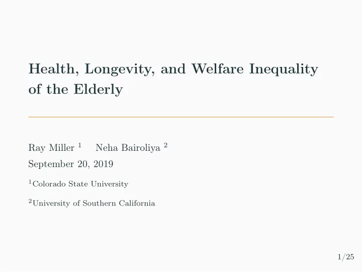
Health, Longevity, and Welfare Inequality

• f the Elderly

Ray Miller 1 Neha Bairoliya 2 September 20, 2019

1Colorado State University 2University of Southern California

1/25

Introduction

Income Gini coefficient by age of family head, 1979-2012

Source: Bosworth, B., Burtless, G., and Zhang, K. (2016). Data from Census Bureau’s Annual Social and Economic Supplement files from the CPS. An “aged head” is 62 years old or older.

2/25

Disparities in well-being

• Consumption and income inequality are incomplete metrics of

well-being

• Leisure, social interactions, political/natural environments, etc.

(e.g. Stiglitz, Sen, and Fitoussi, 2008)

• Health disparities of particular importance among elderly (e.g.

Deaton and Paxson, 1998)

3/25

Mortality rate ratios of low-earning to high-earning men

Source: Bosworth, B., Burtless, G., and Zhang, K. (2016). “Low-earnings” male is one with at least one-half of years of nonzero earnings between ages 41 and 50 in which earnings are below the 31 percentile of male earnings. Data from Survey of Income and Program Participation (SIPP).

4/25

Last age with earnings by thirds of career earnings

Source: Bosworth, B., Burtless, G., and Zhang, K. (2016). Data from Social Security earnings

• records. Career earnings are computed as the average of non-zero earnings for the ages of

41-50. 1943-45 birth cohorts.

5/25

A measure of elderly welfare

• We propose a measure of well-being inequality for the elderly
• Include consumption, leisure, mortality, and health

6/25

A measure of elderly welfare

• We propose a measure of well-being inequality for the elderly
• Include consumption, leisure, mortality, and health
• Standard utility theory provides a useful lens to compare

well-being inclusive of multiple dimensions

6/25

A measure of elderly welfare

• We propose a measure of well-being inequality for the elderly
• Include consumption, leisure, mortality, and health
• Standard utility theory provides a useful lens to compare

well-being inclusive of multiple dimensions

• Recently advocated to adjust GDP across countries (Becker et al.,

2005; Fleurbaey and Gaulier, 2009; Jones and Klenow, 2016)

6/25

A measure of elderly welfare

• We propose a measure of well-being inequality for the elderly
• Include consumption, leisure, mortality, and health
• Standard utility theory provides a useful lens to compare

well-being inclusive of multiple dimensions

• Recently advocated to adjust GDP across countries (Becker et al.,

2005; Fleurbaey and Gaulier, 2009; Jones and Klenow, 2016)

• Welfare measured in income (consumption) equivalents

6/25

A measure of elderly welfare

• We propose a measure of well-being inequality for the elderly
• Include consumption, leisure, mortality, and health
• Standard utility theory provides a useful lens to compare

well-being inclusive of multiple dimensions

• Recently advocated to adjust GDP across countries (Becker et al.,

2005; Fleurbaey and Gaulier, 2009; Jones and Klenow, 2016)

• Welfare measured in income (consumption) equivalents
• Our approach:
• Individual life-cycle simulations =

⇒ entire distribution of welfare

6/25

A measure of elderly welfare

• We propose a measure of well-being inequality for the elderly
• Include consumption, leisure, mortality, and health
• Standard utility theory provides a useful lens to compare

well-being inclusive of multiple dimensions

• Recently advocated to adjust GDP across countries (Becker et al.,

2005; Fleurbaey and Gaulier, 2009; Jones and Klenow, 2016)

• Welfare measured in income (consumption) equivalents
• Our approach:
• Individual life-cycle simulations =

⇒ entire distribution of welfare

• Expected lifetime utility at age 60 =

⇒ ex-ante welfare

6/25

A measure of elderly welfare

• We propose a measure of well-being inequality for the elderly
• Include consumption, leisure, mortality, and health
• Standard utility theory provides a useful lens to compare

well-being inclusive of multiple dimensions

• Recently advocated to adjust GDP across countries (Becker et al.,

2005; Fleurbaey and Gaulier, 2009; Jones and Klenow, 2016)

• Welfare measured in income (consumption) equivalents
• Our approach:
• Individual life-cycle simulations =

⇒ entire distribution of welfare

• Expected lifetime utility at age 60 =

⇒ ex-ante welfare

• Birth cohort analysis =

⇒ not cross-sectional extrapolation

6/25

A measure of elderly welfare

• We propose a measure of well-being inequality for the elderly
• Include consumption, leisure, mortality, and health
• Standard utility theory provides a useful lens to compare

well-being inclusive of multiple dimensions

• Recently advocated to adjust GDP across countries (Becker et al.,

2005; Fleurbaey and Gaulier, 2009; Jones and Klenow, 2016)

• Welfare measured in income (consumption) equivalents
• Our approach:
• Individual life-cycle simulations =

⇒ entire distribution of welfare

• Expected lifetime utility at age 60 =

⇒ ex-ante welfare

• Birth cohort analysis =

⇒ not cross-sectional extrapolation

• Map health to utility =

⇒ quality-adjusted life year (QALY)

6/25

Empirical objectives

• 1. How much better do we expect remaining life to be for the

median sixty year old in the U.S., compared to the sixty year

• ld who is the worst off?

7/25

Empirical objectives

• 1. How much better do we expect remaining life to be for the

median sixty year old in the U.S., compared to the sixty year

• ld who is the worst off?
• 2. How much of the difference in well-being is driven by expected

gaps in consumption versus gaps in leisure or health?

7/25

Empirical objectives

• 1. How much better do we expect remaining life to be for the

median sixty year old in the U.S., compared to the sixty year

• ld who is the worst off?
• 2. How much of the difference in well-being is driven by expected

gaps in consumption versus gaps in leisure or health?

• 3. How has the distribution of elderly welfare changed over time?

7/25

Empirical objectives

• 1. How much better do we expect remaining life to be for the

median sixty year old in the U.S., compared to the sixty year

• ld who is the worst off?
• 2. How much of the difference in well-being is driven by expected

gaps in consumption versus gaps in leisure or health?

• 3. How has the distribution of elderly welfare changed over time?
• 4. How well do other measures (e.g. age 60 income, health)

compare to a (more) complete metric of well-being? What measures best identify well-being gaps?

7/25

Analysis outline

• Welfare model =

⇒ expected utility framework

8/25

Analysis outline

• Welfare model =

⇒ expected utility framework

• Application using Health and Retirement Study (HRS) data
• 1. Forecasting outcomes =

⇒ system of dynamic equations describing the joint evolution of outcomes (panel VAR)

8/25

Analysis outline

• Welfare model =

⇒ expected utility framework

• Application using Health and Retirement Study (HRS) data
• 1. Forecasting outcomes =

⇒ system of dynamic equations describing the joint evolution of outcomes (panel VAR)

• 2. Estimate parameters using full sample

8/25

Analysis outline

• Welfare model =

⇒ expected utility framework

• Application using Health and Retirement Study (HRS) data
• 1. Forecasting outcomes =

⇒ system of dynamic equations describing the joint evolution of outcomes (panel VAR)

• 2. Estimate parameters using full sample
• 3. Age 60 data as initial conditions =

⇒ repeatedly simulate

• utcome paths for each individual

8/25

Analysis outline

• Welfare model =

⇒ expected utility framework

• Application using Health and Retirement Study (HRS) data
• 1. Forecasting outcomes =

⇒ system of dynamic equations describing the joint evolution of outcomes (panel VAR)

• 2. Estimate parameters using full sample
• 3. Age 60 data as initial conditions =

⇒ repeatedly simulate

• utcome paths for each individual
• 4. Derive distribution of ex-ante welfare at age 60
• Four birth cohorts =

⇒ EHRS, LHRS, War Babies, Baby Boomers

8/25

Welfare Model

Welfare model

• Expected lifetime utility:

E J

• a=j

ψiaβa−ju (cia, lia, hia)

• Flow utility: u (c, l, h) = φ (h) [¯

u + log (c) + ν (l)]

Decomposition

9/25

Welfare model

• Expected lifetime utility:

E J

• a=j

ψiaβa−ju (cia, lia, hia)

• Flow utility: u (c, l, h) = φ (h) [¯

u + log (c) + ν (l)]

• φ (h) ∈ [0, 1] =

⇒ quality-adjusted life year (QALY)

Decomposition

9/25

Welfare model

• Expected lifetime utility:

E J

• a=j

ψiaβa−ju (cia, lia, hia)

• Flow utility: u (c, l, h) = φ (h) [¯

u + log (c) + ν (l)]

• φ (h) ∈ [0, 1] =

⇒ quality-adjusted life year (QALY)

• Consumption equivalent welfare λ :

Uij (λ) = E J

• a=j

ψiaβa−ju (λcia, lia, hia)

• welfare defined by:

Umj (λij) = Uij (1)

Decomposition

9/25

Data, Estimation, and Simulation

Data

• Health and Retirement Study (HRS)
• Biennial longitudinal survey of individuals aged 50+ (1992-2014)
• Consumption data (CAMS) on off years (2001-2013)
• Estimation sample
• 35,889 individuals
• 216,626 person-year
• bservations
• Simulation sample (age 60)
• 3,091 EHRS cohort (1931-36)
• 3,607 LHRS cohort (1937-41)
• 2,572 War Babies (1942-47)
• 2,735 Baby Boomers (1948-53)
• Descriptives

10/25

Forecasting model

Time t t + 1 Mt Hypertension Diabetes Lung Disease Heart Disease Stroke Psyche Prob Arthritis ADL Difficulty Self-rated Health (st) Labor Supply (lt) Consumption (ct) Survival (ψt+1) Mt+1, st+1, lt+1, ct+1, ψt+2 Contemporaneous effects Dynamic effects

11/25

Forecasting model

• Structural panel VAR representation:

AYit = BYit−1 + CXit + ǫit

12/25

Forecasting model

• Structural panel VAR representation:

AYit = BYit−1 + CXit + ǫit

• Key assumptions:
• Block triangulation of the system
• Consumption fixed effect
• Differences across cohorts:
• linear time trend
• cohort specific intercept
• initial (age 60) conditions

12/25

Impulse response to onset of heart disease at age 62

5 10 15 Percentage change 60 70 80 90 100 Age Hypertension Diabetes Cancer Lung disease 5 10 15 Percentage change 60 70 80 90 100 Age Stroke Psyche Arthritis ADLs

Notes: Results plot percentage difference in expected outcomes with the exogenous onset of heart disease at age sixty-two relative to remaining without heart disease at sixty-two. Sample includes all individuals in the simulation sample without heart disease at age sixty. Expected

• utcomes are conditional on survival.

13/25

Impulse response to onset of heart disease at age 62

• 20

20 40 60 80 Percentage change 60 70 80 90 100 Age Excellent health Poor health Mortality

• 2
• 1

1 2 3 Percentage change 60 70 80 90 100 Age Consumption Retirement

Notes: Results plot percentage difference in expected outcomes with the exogenous onset of heart disease at age sixty-two relative to remaining without heart disease at sixty-two. Sample includes all individuals in the simulation sample without heart disease at age sixty. Expected

• utcomes are conditional on survival.

Point Estimates

14/25

Life-cycle model fit

Simulated Data

.1 .2 .3 .4 60 65 70 75 80 60 65 70 75 80 60 65 70 75 80 60 65 70 75 80 Early HRS Late HRS War Babies Baby Boomers Heart disease Age .05 .1 60 65 70 75 80 60 65 70 75 80 60 65 70 75 80 60 65 70 75 80 Early HRS Late HRS War Babies Baby Boomers Mortality rate Age .5 1 60 65 70 75 80 60 65 70 75 80 60 65 70 75 80 60 65 70 75 80 Early HRS Late HRS War Babies Baby Boomers Retired Age 22 24 26 28 30 60 65 70 75 80 60 65 70 75 80 60 65 70 75 80 60 65 70 75 80 Early HRS Late HRS War Babies Baby Boomers Consumption ($1000s) Age

Simulated Data 15/25

Calibration of welfare model

• Median 60 year-old in EHRS cohort as reference person
• Health utility function: φ (h) = γh =

⇒ Health Utilities Mark 3 (HUI3)

Results

• Leisure utility function: ν (l) = − θǫ

1+ǫ (1 − l)

1+ǫ ǫ =

⇒ constant Frisch elasticity of labor supply

• ǫ = 1, θ = 8.37 =

⇒ FOC of labor supply holds at median

• Working =

⇒ l = 0.66

• Discount factor β = 0.98
• Flow utility intercept ¯

u = −0.34 = ⇒ median value of remaining life equal to $50,000 per QALY

16/25

Welfare Results

Elderly welfare inequality

Welfare Gini 10/50 ratio 90/50 ratio ρ Benchmark 0.544 0.234 3.774

• No morbidity

0.453 0.335 2.831 0.972

Notes: Estimates use base year sampling weights. No morbidity measure removes health from flow utility. Spearman’s rank correlation between the two welfare measures denoted by ρ.

.1 .2 .3 .4 .5 Density

• 5

5 Log welfare Benchmark No morbidity

Dollar Value QALE

17/25

Elderly welfare and decomposition by decile

More

• 200
• 100

100 200 Mean log points 10 9 8 7 6 5 4 3 2 1

Welfare decile

Welfare Consumption QALE Leisure 18/25

Life-cycle profiles by welfare decile

20 40 60 $1000s 60 70 80 90 Age

Consumption

.8 .85 .9 .95 1 Fraction of time endowment 60 70 80 90 Age

Leisure

.4 .5 .6 .7 .8 .9 Fraction of full health 60 70 80 90 Age

Health utility

.2 .4 .6 .8 1 Cumulative mortality probability 60 70 80 90 Age

Mortality Lowest (1st) Decile 5th Decile Highest (10th) Decile

19/25

Welfare over cohorts

Cohort Gini 10/50 ratio 90/50 ratio EHRS 0.544 0.234 3.774 LHRS 0.606 0.210 4.667 War Babies 0.643 0.196 5.159 Baby Boomers 0.674 0.196 5.727

Notes: Estimates use base year respondent analysis weights. Robustness

20/25

Welfare over cohorts

.1 .2 .3 .4 Density

• 5

5 Log welfare .2 .4 .6 Density 2 4 6 8 10 Log expected lifetime consumption .02 .04 .06 .08 Density 10 20 30 40 Life expectancy .02 .04 .06 .08 Density 10 20 30 QALE

EHRS LHRS War Babies Baby Boomers

21/25

Comparison with other measures of well-being

Measure Gini ρ Welfare (λ) 0.544 Income 0.492 0.508 Consumption 0.424 0.573 Health utility 0.109 0.745 Flow utility 0.235 0.767 Life expectancy 0.132 0.818 QALE 0.176 0.872 Expected lifetime consumption 0.364 0.921

Notes: Estimates for initial HRS cohort using base year respondent analysis weights. Income, consumption, and health utility are cross-sectional measures at age sixty. Flow utility is calculated using cross-sectional consumption, leisure, and health along with our benchmark

• preferences. Spearman’s rank correlation between λ and each measure denoted by ρ.

Graphs

22/25

Comparison with other measures of over cohorts

Cohort Welfare (λ) Cons. QALE ELC EHRS 0.544 0.424 0.184 0.364 LHRS 0.606 0.442 0.198 0.390 War Babies 0.643 0.443 0.203 0.403 Baby Boomers 0.674 0.449 0.215 0.427

Notes: Estimates use base year respondent analysis weights. Income, consumption, and health utility are cross-sectional measures at age sixty. QALE is quality-adjusted life expectancy at age sixty. ELC is expected lifetime consumption at age sixty.

23/25

Conclusions

• 1. Elderly welfare inequality is substantial
• Driven foremost by health and mortality gaps, followed by gaps

in consumption

• Ignoring well-being cost of health significantly underestimates

inequality

24/25

Conclusions

• 1. Elderly welfare inequality is substantial
• Driven foremost by health and mortality gaps, followed by gaps

in consumption

• Ignoring well-being cost of health significantly underestimates

inequality

• 2. Welfare inequality has increased over time
• Growing gaps in consumption, health, and mortality

24/25

Conclusions

• 1. Elderly welfare inequality is substantial
• Driven foremost by health and mortality gaps, followed by gaps

in consumption

• Ignoring well-being cost of health significantly underestimates

inequality

• 2. Welfare inequality has increased over time
• Growing gaps in consumption, health, and mortality
• 3. Cross-sectional income and consumption at age 60
• Underestimate the level and growth of aggregate inequality
• Are worse predictors of individual welfare rank than

cross-sectional health

24/25

Limitations and future work

• Limitations
• Abstract from potentially important inputs =

⇒ caregiver time, social interactions, end-of-life care, bequests, etc.

• Single set of preferences
• Forecasting model falls short of fully specified structural model
• Opportunities for future work
• Sub-sample analysis (e.g. education, race, gender, age)

Maps

• Policy experiments / outcome in natural experiments
• Cross-country comparison of elderly welfare inequality

25/25

Thank You!

25/25

Welfare decomposition

Back

log (λij) =

˜ ψ

J

• a=j

βa−j [(E [ψiaφ (hia)] − E [ψmaφ (hma)]) E [uia] + Φ] QALE + ˜ ψ

J

• a=j

βa−jE [ψmaφ (hma)] (E [log (cia)] − E [log (cma)]) Cons. + ˜ ψ

J

• a=j

βa−jE [ψmaφ (hma)] (E [ν (lia)] − E [ν (lma)]) Leisure

where

Φ = (E [ψiaφ (hia) uia] − E [ψiaφ (hia)] E [uia]) − (E [ψmaφ (hma) uma] − E [ψmaφ (hma)] E [uma])

25/25

Simulation sample initial conditions by cohort

Back EHRS LHRS WB BB Age (mean) 60 60 60 60 Hypertension (%) 38.10 41.93 47.60 51.23 Diabetes (%) 11.81 12.77 16.45 20.13 Cancer (%) 6.84 8.25 10.82 9.48 Lung disease (%) 7.11 6.78 7.37 8.15 Heart disease (%) 13.85 14.75 16.11 16.25 Stroke (%) 2.90 3.88 5.22 4.66 Psyche problem (%) 7.44 11.85 17.32 21.85 Arthritis (%) 44.79 48.12 51.62 52.53 Difficulty with ADLs (%) 11.75 19.35 22.40 22.42 Self-rated health (%) Poor 7.31 6.68 6.61 7.26 Fair 15.20 16.71 16.60 17.15 Good 28.32 30.12 31.08 29.34 Very good 31.66 30.80 31.72 34.19 Excellent 17.51 15.70 13.98 12.06 Retired (%) 48.66 50.46 48.07 47.47 Annual consumption ($1000s, mean) 27.59 30.29 29.43 26.41

Notes: Mean and percentage estimates use base year sampling

• weights. Consumption is reported in real 2010 dollars.

25/25

Select estimation results

Back

Hypertension Diabetes Cancer Lung Disease Heart Disease Stroke Psyche Problem Arthritis Difficulty with ADLs Good Health Retired 0.04 0.08 Poor health

• .3 -.2 -.1 0 .1 .2

Retirement

• .1-.05 0 .05 .1

Log consumption

• .1 -.05 0 .05 .1

Mortality

• .02-.01 0 .01 .02

Stroke

Notes: Dependent variables across columns. Average marginal effects on the probability of an

• utcome reported for probit results—poor health, retirement, mortality, and stroke.

Contemporaneous associations reported for poor health, retirement, and consumption as dependent variables. Lagged associations reported for mortality and stroke. Good health coefficients use poor health state as reference group. Spikes indicate 95% confidence intervals.

25/25

Estimated health utility weights

Back

Measure Weight SE Self-rated health Fair 0.226 0.026 Good 0.313 0.026 Very good 0.403 0.027 Excellent 0.421 0.031 Hypertension 0.003 0.012 Diabetes

• 0.001

0.018 Cancer 0.010 0.017 Lung disease

• 0.020

0.022 Heart disease

• 0.032

0.015 Stroke

• 0.076

0.022 Psych problem

• 0.073

0.020 Arthritis

• 0.062

0.012 Diff with ADL

• 0.161

0.016 Constant 0.517 0.028 Notes: Results from regression of HUI3 score on self-rated health and morbidities. SE denotes standard error. R2 = 0.48. N = 1,089. 25/25

Quality adjusted life expectancy

Back

.2 .4 .6 .8 1 Ratio of QALE to Life Expectancy 10 20 30 40 Life Expectancy 25/25

Age 60 Consumption and QALE by welfare decile

Back

20 40 60 80 100+ Consumption ($1000s) 10 20 30 QALE Lowest Decile Highest Decile 25/25

Robustness

Back

Gini by cohort Measure λ 10/50 λ 90/50 EHRS LHRS WB BB ρ Benchmark 0.234 3.774 0.544 0.606 0.643 0.674 0.573 Compensating variation 0.059 2.856 0.505 0.533 0.546 0.566 0.556 Reference 90th %tile 0.314 2.842 0.446 0.500 0.533 0.555 0.573 $100k per QALY 0.076 6.465 0.670 0.731 0.763 0.784 0.502 β = 0.90 0.256 3.130 0.491 0.539 0.567 0.590 0.616 ǫ = 0.5 0.231 3.726 0.539 0.600 0.637 0.665 0.572 ǫ = 2 0.239 4.074 0.560 0.620 0.658 0.692 0.570 θ = 15.9 0.258 3.539 0.525 0.584 0.621 0.652 0.571 Survival adjusted 0.177 4.015 0.568 0.618 0.648 0.674 0.573 Non-imputed data 0.242 3.543 0.522 0.568 0.591 0.627 0.603

Notes: Estimates use base year respondent analysis weights. War Babies denoted by WB and Baby Boomers by BB. Spearman’s rank correlation between welfare and cross-sectional consumption at age sixty denoted by ρ.

25/25

Robustness

Back

• More general preferences:

u (c, l, h) = φ (h)

• ¯

u + c1−γ 1 − γ

• 1 − (1 − γ)

θǫ 1 + ǫ (1 − l)

1+ǫ ǫ

γ − 1 1 − γ

• EV 10/50 ratio by cohort

CV 90/50 ratio by cohort EHRS LHRS WB BB EHRS LHRS WB BB ρ γ = 1 0.234 0.210 0.196 0.196 2.856 3.161 3.211 3.563 0.573 γ = 1.5 0.207 0.180 0.163 0.165 3.567 3.915 3.829 4.158 0.520 γ = 2 0.231 0.197 0.163 0.167 4.237 4.500 4.183 4.502 0.471

Notes: Estimates use base year respondent analysis weights. War Babies denoted by WB and Baby Boomers by BB. Spearman’s rank correlation between EV measure of welfare and cross-sectional consumption at age sixty denoted by ρ.

25/25

Welfare and age 60 income/health

Back

20 40 60 80 100+ Income ($1000s) 1 2 3 4 5+ Welfare .2 .4 .6 .8 1 Health utility 1 2 3 4 5+ Welfare

25/25

Welfare by census division for HRS cohort

Back

Median Welfare

1.4 - 1.6 1.1 - 1.4 .8 - 1.1 .6 - .8

Welfare 90/10 Ratio

19 - 20 16 - 19 15 - 16 14 - 15 13 - 14 12 - 13

25/25

Welfare decomposition in EHRS cohort

Back

Decomposition Median λ Mean log λ Cons. Leisure QALY Education <HS 0.444

• 0.802
• 0.393

0.031

• 0.440

HS grad 1.058

• 0.020
• 0.015

0.019

• 0.025

Some college 1.402 0.271 0.196 0.006 0.069 College grad 2.536 0.893 0.476

• 0.012

0.429 Gender Male 0.862

• 0.150

0.045

• 0.005
• 0.190

Female 1.182 0.083

• 0.030

0.031 0.081 Race White 1.112 0.070 0.063 0.013

• 0.005

Black 0.457

• 0.742
• 0.404

0.028

• 0.366

Other 0.771

• 0.304
• 0.245

0.011

• 0.070

25/25

Welfare Dollar Value

Back

50 100 150 200 250 $1000s 1 2 3 4 5 6 7 8 9 10

Consumption by Welfare Decile

Age 60 Consumption Age 60 Equivalent Consumption 25/25

Welfare Dollar Value

Back

• 1000
• 500

500 Mean Willingness to Pay 1 2 3 4 5 6 7 8 9 10 Welfare decile $1,000s $10,000s 25/25