Head Motion Prediction in Augmented Reality Systems Using Monte - PDF document
ICAT 2003 December 3-5, Tokyo, JAPAN Head Motion Prediction in Augmented Reality Systems Using Monte Carlo Particle Filters Fakhr-eddine Ababsa, Jean Yves Didier, Malik Mallem, David Roussel Laboratoire Systmes Complexes. CNRS FRE 2494 40,
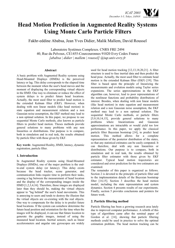
ICAT 2003 December 3-5, Tokyo, JAPAN Head Motion Prediction in Augmented Reality Systems Using Monte Carlo Particle Filters Fakhr-eddine Ababsa, Jean Yves Didier, Malik Mallem, David Roussel Laboratoire Systèmes Complexes. CNRS FRE 2494 40, Rue du Pelvoux, CE1455-Courcouronnes 91020 Evry Cedex France [ababsa | didier | mallem | roussel] @iup.univ-evry.fr used for head motion tracking [12,13,18,20,21]. A filter Abstract structure is used to fuse inertial data and then predict the A basic problem with Augmented Reality systems using head pose. Actually, the most used filter to estimate head Head-Mounted Displays (HMDs) is the perceived motion is the extended Kalman filter (EKF) [19]. This latency or lag. This delay corresponds to the elapsed time filter is based upon the principle of linearizing the between the moment when the user's head moves and the measurements and evolution models using Taylor series moment of displaying the corresponding virtual objects expansions. The series approximations in the EKF in the HMD. One way to eliminate or reduce the effect of algorithm can, however, lead to poor representations of system delays is to predict future head locations. the nonlinear functions and probability distributions of Actually, the most used filter to predict head motion is interest. Besides, when dealing with non linear models the extended Kalman filter (EKF). However, when (like head motion) in state equation and measurement dealing with non linear models (like head motion) in relation and a non Gaussian noise assumption, the EKF state equation and measurement relation and a non method may lead to a non optimal solution. The Gaussian noise assumption, the EKF method may lead to sequential Monte Carlo methods, or particle filters a non optimal solution. In this paper, we propose to use [5,9,10,14,15], provide general solutions to many sequential Monte Carlo methods, also known as particle problems where linearizations and Gaussian filters to predict head motion. Theses methods provide approximations are intractable or would yield too low general solutions to many problems with any non performance. In this paper, we apply the classical linearities or distributions. Our purpose is to compare, particle filter Bayesian bootstrap [14], to predict head both in simulation and in real task, the results obtained motion. This method allows for a complete by particle filter with those given by EKF. representation of the posterior distribution of the states, so that any statistical estimates can be easily computed. It Key words : Augmented Reality, HMD, latency, dynamic can therefore, deal with any non linearities or registration, particle filter. distributions. Our purpose is to compare, both in simulation and in real task, the results obtained by 1. Introduction particle filter estimator with those given by EKF estimator. Typical head motion trajectories are In Augmented Reality systems using Head-Mounted considered and error prediction for the two estimators are Displays (HMDs), one of the major problem is the end- examined. to-end system delay (or latency). This delay exists The remainder of this paper is organized as follows. because the head tracker, scene generator, and Section 2 is devoted to the principle of particle filter and communication links require time to perform their tasks, to the implementation details of the Bayesian bootstrap causing a lag between the measurement of head location filter [14,15]. Section 3 describes the head motion and the display of the corresponding images inside the model, including the state representation and system HMD [1,2,3,4,16]. Therefore, those images are displayed dynamics. Section 4 presents results of our experiments. later than they should be, making the virtual objects Finally, section 5 provides conclusions and pointers for appear to "lag behind" the user's head movements. This future work. is annoying to users and tends to destroy the illusion that the virtual objects are co-existing with the real objects. 2. Particle filtering method One way to compensate for the delay is to predict future head locations. If the system can somehow determine the Particle filtering has been a growing research area lately future head position and orientation for the time when the due to improved computer performance. A rebirth of this images will be displayed, it can use that future location to type of algorithms came after the seminal paper of generate the graphic images, instead of using the Gordon et al. [14], showing that particle filtering measured head location. Inertial sensors, such as linear methods could be used in practice to solve the optimal accelerometers and angular rate gyroscopes are widely estimation problem. The head motion tracking can be
( ) considered as a single target non linear discrete time ( i ) ( i *) 4. Predict new particles, i.e, x f x , v , = t + 1 t t system: i = 1,…,N using different noise realization for the ( ) x f x , v = particles. t 1 t 1 t + − (1) ( ) y h x e 5. Increase t and iterate to item 2. = + t t t The particle filters provide an approximative Bayesian 3. Head motion model and system dynamics solution to discrete time recursive problem by updating an approximative description of the posterior filtering Our AR tracking system consists of a robust vision n density. Let x denote the state of the observed landmark tracker and an inertial measurement unit (IMU) ∈ ℜ t providing 3D linear acceleration and 3D rate of turn (rate { } t system and Y y be the set of observations until = t i i 0 = gyro). The 3D coordinate frames used in our study, as present time. Assume independent process noise v t and illustrated in figure (1), are: {W} the world coordinate measurement noise e t with densities p vt respective p et . system, {C} the camera-centered coordinate system, and The initial uncertainty is described by the density p x0 . {I} the inertial-centered coordinate system. Since the The particle filter approximates the probability density inertial sensor is rigidly mounted to the camera, the p(x t |Y t ) transformation between the camera frame {C} and the by a large set of N particles { } N inertial frame {I} is known. ( i ) x = , where each particle t i 1 ( i ) Inertial/camera frames has an assigned relative weight, w , such that all t weights sum to unity. The location and weight of each World frame C particle reflect the value of the density in the region of I the state space. The particle filter updates the particle location and the corresponding weights recursively with W each new observation. The non-linear prediction density p(x t |Y t-1 ) and filtering density p(x t |Y t ) for the Bayesian interference are given by: Fig. 1 Frames of reference ( ) ( ) ( ) p x Y p x x p x Y dx (2) = − � t t 1 t t 1 t 1 t 1 t 1 − − − − We used head motion model proposed by Chai et al. n ℜ [6,7], where head motion is represented by 15 × 1 vector: ( ) ( ) ( ) p x Y p y x p x Y (3) − ∝ t t 1 t t t t − 1 ( ) X head , , x , x , x (6) = θ ω � � � The main idea is to approximate p(x t |Y t-1 ) with where θ θ is the orientation of the camera frame with θ θ N ( ) ( ) respect to the world (we use Z-Y-X Euler angles), ω ω is ω ω ( i ) 1 p x Y x x (4) ≈ δ − t t 1 � t t − N the angular velocity , and x , x , x are the position, � � � i 1 = velocity, and acceleration of the camera with respect to where δ is the discrete Dirac function. Inserting equation the world. With these states, the discretized system (4) into equation (3) yields a density to sample from. dynamics are given by [6]: This can be done by using the Bayesian bootstrap or Sampling Importance Resampling (SIR) algorithm from ( ) 1 θ T W v θ + ∆ ⋅ θ ⋅ ω + � � � � [14], given in Table (1). k 1 + k k k � � � � The estimate for the particle filter can be calculated as : � � 2 � � ω v ω + k 1 N + k k � � � � N ( i ) ( i ) ˆ x w x (5) = � � � � t � t t 2 3 x 1 (7) = x T x T x v + ∆ ⋅ + ∆ ⋅ + � � � � � � � i 1 = k 1 + k k 2 k k � � � � Table 1. Bayesian bootstrap (SIR) algorithm � � � � 4 x x T x v � + ∆ ⋅ + � � � 1. Set t=0, generates N samples { } N k 1 + � k k k � ( i ) x = from the � � 0 i 1 � � � � 5 x x v initial distribution p(x 0 ). � � + � � � � � � k 1 + k k � � � � ( ) ( i ) ( i ) 2. Compute the weights w = p y x and t t t where ∆ T is the sampling period, W( θ ) is the Jacobian N matrix that relates the absolute rotation angle to the ~ ( i ) ( i ) ( j ) normalize, i.e, w w w , i 1 ,.... N . = = i t t � t angular rate [8], and v are the system random k j 1 = distribution noise. 3. Generate a new set { } N ( i *) x = by resampling with Otherwise, sensors have associated with them an output t i 1 equation, which maps the states to the sensor output. replacement N times from { } N ( i ) x , where Since the goal of our study is to compare performances 0 i 1 = ( ) ~ ( i *) ( j ) ( j ) of a particle filter estimator and an EKF estimator, we Pr x x w . = = t t t suppose that observation equations measure directly the
Recommend
More recommend
Explore More Topics
Stay informed with curated content and fresh updates.
