GRAPH REPRESENTATIONS, BACKPROPAGATION AND BIOLOGICAL PLAUSIBILITY - PowerPoint PPT Presentation

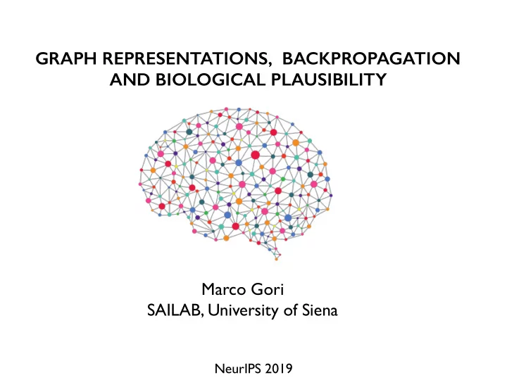
GRAPH REPRESENTATIONS, BACKPROPAGATION AND BIOLOGICAL PLAUSIBILITY Marco Gori SAILAB, University of Siena NeurIPS 2019

OUTLINE • Learning in structured domains • Diffusion machines and spatiotemporal locality • Backpropagation diffusion and biological plausibility NeurIPS 2019

LEARNING IN STRUCTURED DOMAINS ? NeurIPS 2019

Graphs as Pattern Models r o i v a h image classification e b l a c i m e h c o c i s y h p What are the features?

Social nets quasi-eqlibrium dynamic models here we need to make prediction at node level! Social networks Citation networks Communication networks Multi-agent systems

GRAPH NEURAL NETS popular and successful mostly thanks to ? graph convolutional networks pictures from Z. Wu et al Non-Euclidean Deep Learning NeurIPS 2019

HISTORICALLY … ANOTHER PATH WAS FOLLOWED! NeurIPS 2019

Extension of the idea of time unfolding …

Structure unfolding The case of binary trees …

5 59 510 56 57 58 55 51 52 53 54 39 310 49 410 36 37 38 46 47 48 35 45 31 32 33 34 41 42 43 44 NeurIPS 2019 The Graph Neural Network Model 19 110 29 210 A recurrent net arises from cyclic graphs 16 17 18 26 27 28 Gori et al IJCNN 2005, 2009 IEEE-TNN Graph Compiling … 15 25 11 12 13 14 21 22 23 24 5 59 510 56 57 58 39 310 55 49 410 36 37 38 46 47 48 19 110 35 29 210 45 16 17 18 26 27 28 15 25 11 12 13 14 23 24 25

LEARNING AS A DIFFUSION PROCESS THE FRAMEWORK OF CONSTRAINED-BASED LEARNING AND THE ROLE OF TIME COHERENCE ? NeurIPS 2019

Natural Laws of Learning there is no distinction between training and test sets! Once we believe in ergodicity … The links with mechanics laws of learning regularization term Loss function of neural net Z T ✓ 1 ◆ q 2 + 1 q 2 + V ( q, t ) dt e − t/ ✏ 2 ✏ 2 ⇢ ¨ A = 2 ✏⌫ ˙ ✏ 0 laws of mechanics kinetic energy potential energy NeurIPS 2019

Natural Laws of Cognition: A Pre-Algorithmic Step Natural Learning Theory � Mechan- Remarks s a ics t w i � q i e Weights are interpreted as generalized coor- n dinates. s l e a w i � ˙ Weights variations are interpreted as gener- l ˙ q i r c u i alized velocities. t e r n a υ i � p i The conjugate momentum to the weights is p f o defined by using the machinery of Legendre n s o transforms. t i h t A(w) � S(q) g i The cognitive action is the dual of the action s i o e in mechanics. p w w) � L(t, q, ˙ The Lagrangian F is associated with the F(t, w, ˙ q) classic Lagrangian L in mechanics. H(t, w, υ ) � H(t, q, p) When using w and υ , we can define the Hamiltonian, just like in mechanics. NeurIPS 2019

Constraint Reactions architectural and environmental constraints ∧ ∨ L = { (( 0 , 0 ), 0 ), (( 0 , 1 ), 1 ), (( 1 , 0 ), 1 ), (( 1 , 1 ), 0 ) } = 1 2 y ((0 , 1) , (1 , 0)) ¬ y ((0 , 0) , (1 , 1)) . 3 4 “hard” architectural constraints x κ 3 − σ ( w 31 x κ 1 + w 32 x κ 2 + b 3 ) = 0 x κ 4 − σ ( w 41 x κ 1 + w 42 x κ 2 + b 4 ) = 0 κ = 1 , 2 , 3 , 4 x κ 5 − σ ( w 53 x κ 3 + w 54 x κ 4 + b 4 ) = 0 training set constraints x 15 = 1 , x 25 = 1 , x 35 = 0 , x 45 = 0 NeurIPS 2019

Lagrangian Approach variational calculus under subsidiary conditions Lagrangian Multipliers functional optimization: Static Models Dynamic Models holonomic constraints non-holonomic constraints

Formulation of Learning holonomic constraints (DAGs) R regularization term risk function Z 1 x ( t ) | 2 + m W | ˙ W ( t ) | 2 ) $ ( t ) dt + F ( x, W ) , A ( x, W ) := 2( m x | ˙ ∈ M # let us consider the case and let constraints ν x, W, ˙ W, ¨ R wing F ( x, W ) := F ( t, x, ˙ x, ¨ W ) dt , G j ( t, x ( t ) , W ( t )) = 0 , 1 ≤ j ≤ ⌫ . neural constraints (Einstein’s notation) proposition holds true: ⇢ ⇠ j − e j ( ⌧ ) , if 1 ≤ j ≤ ! ; G j ( ⌧ , ⇠ , M ) := ⇠ j − � ( m jk ⇠ k ) if ! < j ≤ ⌫ , Proposition 1 : Functionally independent for acyclic graphs feedforward nets

Formulation of Learning (con’t) holonomic constraints - any digraph regularization term risk function Z Z 1 x ( t ) | 2 + m W | ˙ W ( t ) | 2 + m s | ˙ s ( t ) | 2 ) $ ( t ) dt + F ( x, W, s ) , A ( x, W, s ) := 2( m x | ˙ (12) x, W, ˙ W, ¨ R re F ( x, W, s ) := F ( t, x, ˙ x, ¨ W, s ) dt . neural constraints slack variables ( ⇠ j − e j ( ⌧ ) + ⇣ j , if 1 ≤ j ≤ ! ; G j ( ⌧ , ⇠ , M, ⇣ ) := ⇠ j − � ( m jk ⇠ k ) + ⇣ j if ! < j ≤ ⌫ . Proposition 2 : Functionally independent for any graph

Formulation of Learning (con’t) Non-holonomic constraints (any digraph) regularization term loss term Z ⇣ m x x ( t ) | 2 + m W W ( t ) | 2 + F ( t, x, W ) ⌘ 2 | ˙ A ( x, W ) = 2 | ˙ $ ( t ) dt neural constraints x i ( t ) + cx i ( t ) − � ( w ik ( t ) x k ( t )) = 0; ˙ 0 < c < 1 Proposition 3 : Functionally independent for any graph

Feedforward Networks (DAGs) x ( t ) − � j ( t ) G j ξ ( x ( t ) , W ( t )) + L x − m x $ ( t )¨ x ( t ) − m x ˙ $ ( t ) ˙ F ( x ( t ) , W ( t )) = 0; − m W $ ( t ) ¨ $ ( t ) ˙ W ( t ) − � j ( t ) G j M ( x ( t ) , W ( t )) + L W W ( t ) − m W ˙ F ( x ( t ) , W ( t )) = 0 , instantaneous linear equation ξ a G j ⇣ G i + G i m ab G j x a + G i x a ˙ ⌘ ξ a m ab G i ττ + 2( G i w ab + G i � � j = $ τξ a ˙ τ m ab ˙ ξ a m bc ˙ w bc ) m x m W x a ˙ x b + G i + G i � ξ a ξ b ˙ m ab m cd ˙ w ab ˙ w cd L x a F G i + L w ab G i ξ a m ab F x a G i w ab G i − ˙ $ ( ˙ ξ a + ˙ m ab ) + , m x m W where L x x ) /dt + d 2 ( F ¨ x ) /dt 2 , L W W ) /dt + d 2 ( F ¨ W ) /dt 2 F = F x − d ( F ˙ F = F W − d ( F ˙ vatives of F with respect to x and W respectively (see ( 9 )). An expression for Lagrange supervised learning x, W, ˙ W, ¨ W ) = F ( t, x ) → L x L w F ( t, x, ˙ x, ¨ F = ∂ x F, F = 0

Reduction to Backpropagation m x → 0 → W the chain rule arises … W ij = − 1 ˙ � � 0 ( w ik x k ) � i x j ; x ξ a G j G i ξ a � j = − V x a G i ξ a , λ Augmented Learning Space T � = − V x , T is � 3 = − V x 3 ;   − � 0 ( w 21 x 1 ) w 21 1 0 − � 0 ( w 32 x 2 ) w 32 T = 0 1 � 2 = � 0 ( w 32 x 2 ) w 32 � 3 ;   0 0 1 � 1 = � 0 ( w 21 x 1 ) w 21 � 2 . Eq. (26) the Lagrange multipliers are derived as follows A somewhat surprising kinship with the BP delta-error Early discovery by Yan Le Cun, 1989

Augmented Learning Space Euler-Lagrange Equations W non-holonomic constraints x intuition: we need to store the multipliers and provide temporal updating λ x i ( t ) + cx i ( t ) − � ( w ik ( t ) x k ( t )) = 0; ˙ 1 − BP-like GNN factorization δ j x i W ( t ) = − 1 ˙ � � j ( t ) G j M ( t, x ( t ) , W ( t ) , ˙ x ( t )); This makes GNN efficient! ˙ � ( t ) = � j ( t ) G j ξ ( t, x ( t ) , W ( t ) , ˙ x ( t )) + V ξ ( t, x ( t )) Unlike BPTT and RTRL, learning equations are local in space and time: connections with Equilibrium Propagation (Y. Bengio et al)

DIFFUSION LEARNING AND BIOLOGICAL PLAUSIBILITY reactions: Lagrangian multipliers δ i environmental interaction LOCALITY IN SPACE AND IN TIME inputs x j

Biological Plausibility of Backpropagation Biological concerns should not involve BP , BP diffusion is biologically plausible BP algorithm is NOT biologically plausible but the instantaneous map x i ( t ) = σ ( w ik x k ( t )) replace with − x i ( t ) = � ( w ik ( t − 1) x k ( t − 1)) . x i ( t ) + cx i ( t ) − � ( w ik ( t ) x k ( t )) = 0; ˙ … clever related comment by Francis Crick, 1989

Forward and Backward Waves BP diffusion is biologically plausible t + 1 t + 2 t + 3 t + 4 t + 5 t + 6 t + 7 t + 8 t BP algorithm is NOT biologically plausible

Conclusions PRELIMINARY EXPERIMENTAL CHECK • GNN: Success due to convolutional graphs, but the “diffusion path” is still worth exploring • What happens with deep networks in graph compiling? • Laws of learning, pre-algorithmic issues, and biological plausibility • Dynamic models for Lagrangian multipliers (always delta- error): new perspective whenever time-coherence does matter! • Euler-Lagrangian Learning and SGD

Acknowledgments Alessandro Betti, SAILAB Publications • F. Scarselli et al, “The Graph Neural Network Model,” IEEE-TNN, 2009 • A. Betti, M. Gori, and S. Melacci, Cognitive Action Laws: The Case of Visual Features, IEEE-TNNLS 2019 • A. Betti, M. Gori, and S. Melacci, Motion Invariance in Visual Environment, IJCAI 2019 • A. Betti and M. Gori, Backprop Diffusion is Biologically Plausible, arXiv:1912.04635 • A. Betti and M. Gori, Spatiotemporal Local Propagation, arXiv: 1907.05106 Software • arXiv:1912.04635 • Preliminary version NeurIPS 2019

Machine Learning A CONSTRAINT-BASED APPROACH Marco Gori