Graph Representation Learning William L. Hamilton COMP 551 - PowerPoint PPT Presentation
Graph Representation Learning William L. Hamilton COMP 551 Special Topic Lecture Will Hamilton, McGill and Mila 1 Why graphs? Graphs are a general language for describing and modeling complex systems Will Hamilton, McGill and Mila 2
Graph Representation Learning William L. Hamilton COMP 551 – Special Topic Lecture Will Hamilton, McGill and Mila 1
Why graphs? Graphs are a general language for describing and modeling complex systems Will Hamilton, McGill and Mila 2
Will Hamilton, McGill and Mila 3
Graph! Will Hamilton, McGill and Mila 4
Many Data are Graphs Social networks Economic networks Biomedical networks C Information networks: Internet Networks of neurons Web & citations Will Hamilton, McGill and Mila 5
Why Graphs? Why Now? § Universal language for describing complex data § Networks/graphs from science, nature, and technology are more similar than one would expect § Shared vocabulary between fields § Computer Science, Social science, Physics, Economics, Statistics, Biology § Data availability (+computational challenges) § Web/mobile, bio, health, and medical § Impact! § Social networking, Social media, Drug design Will Hamilton, McGill and Mila 6
Machine Learning with Graphs Classical ML tasks ks in graphs: § Node classification § Predict a type of a given node § Link prediction § Predict whether two nodes are linked § Community detection § Identify densely linked clusters of nodes § Network similarity § How similar are two (sub)networks Will Hamilton, McGill and Mila 7
Example: Node Classification ? ? ? ? Machine Learning ? Will Hamilton, McGill and Mila 8
Example: Node Classification Cl Classifying ng the he fu functi ction on of of protei oteins in in the in intera ractome! Image from: Ganapathiraju et al. 2016. Schizophrenia interactome with 504 novel protein–protein interactions. Nature . Will Hamilton, McGill and Mila 9
Example: Link Prediction ? ? x ? Machine Learning Will Hamilton, McGill and Mila 10
Example: Link Prediction Co Cont ntent nt re recommendation is link k prediction! ? Will Hamilton, McGill and Mila 11
Machine Learning Lifecycle § (Supervised) Machine Learning Lifecycle: This feature, that feature. Every single time! Raw Structured Learning Model Data Data Algorithm Automatically Feature Downstream Engineering learn the features prediction task Will Hamilton, McGill and Mila 12
Feature Learning in Graphs Goal: Efficient task-independent feature learning for machine learning in graphs! vec node 2 u !: # → ℝ & ℝ & Feature representation, embedding Will Hamilton, McGill and Mila 13
Example § Zachary’s Karate Club Network: A B In Input Ou Outpu put Image from: Perozzi et al. 2014. DeepWalk: Online Learning of Social Representations. KDD. Will Hamilton, McGill and Mila 14
Why Is It Hard? § Modern deep learning toolbox is designed for simple sequences or grids. § CNNs for fixed-size images/grids…. § RNNs or word2vec for text/sequences… Will Hamilton, McGill and Mila 15
Why Is It Hard? § But graphs are far more complex! § Complex topographical structure (i.e., no spatial locality like grids) § No fixed node ordering or reference point (i.e., the isomorphism problem) § Often dynamic and have multimodal features. Will Hamilton, McGill and Mila 16
This talk § 1) Node embeddings § Map nodes to low-dimensional embeddings. § 2) Graph neural networks § Deep learning architectures for graph- structured data § 3) Example applications. Will Hamilton, McGill and Mila 17
Pa Part rt 1 1: : Node Node Emb Embeddings Will Hamilton, McGill and Mila 18
Embedding Nodes A B In Input Ou Outpu put Intuition: Find embedding of nodes to d- dimensions so that “similar” nodes in the graph have embeddings that are close together. Will Hamilton, McGill and Mila 19
Setup § Assume we have a graph G : § V is the vertex set. § A is the adjacency matrix (assume binary). § No No no node de featur ures or extra inf nformation n is us used! Will Hamilton, McGill and Mila 20
Embedding Nodes • Goal is to encode nodes so that similarity in the embedding space (e.g., dot product) approximates similarity in the original network. Will Hamilton, McGill and Mila 21
Embedding Nodes similarity( u, v ) ≈ z > Go Goal: v z u Ne Need d to de define ne! Will Hamilton, McGill and Mila 22
Learning Node Embeddings ine an encoder (i.e., a mapping from 1. 1. De Defin nodes to embeddings) 2. 2. De Defin ine a node sim imila ilarit ity functio ion (i.e., a measure of similarity in the original network). 3. 3. Op Optimize the parameters of f the encoder so so that: similarity( u, v ) ≈ z > v z u Will Hamilton, McGill and Mila 23
Two Key Components Encoder maps each node to a low-dimensional § En vector. d -dimensional embedding enc ( v ) = z v node in the input graph y function specifies how relationships in § Si Simi milarity vector space map to relationships in the original network. similarity( u, v ) ≈ z > v z u Similarity of u and v in dot product between node the original network embeddings Will Hamilton, McGill and Mila 24
“Shallow” Encoding § Simplest encoding approach: en enco coder er is is ju just an an em embed edding-looku kup enc ( v ) = Zv matrix, each column is node Z ∈ R d × |V| embedding [wh [what we we le learn!] !] indicator vector, all zeroes v ∈ I |V| except a one in column indicating node v Will Hamilton, McGill and Mila 25
“Shallow” Encoding § Simplest encoding approach: en enco coder er is ju is just an embeddin ing-looku kup embedding vector for a specific node embedding matrix Dimension/size Z = of embeddings one column per node Will Hamilton, McGill and Mila 26
“Shallow” Encoding § Simplest encoding approach: en enco coder er is is ju just an an em embed edding-looku kup. i. i.e., each node is is assig igned a uniq ique em embed edding ve vector. § E.g., node2vec, DeepWalk, LINE Will Hamilton, McGill and Mila 27
How to Define Node Similarity? § Key distinction between “shallow” methods is ho how the they define ne no node si similarity. § E.g., should two nodes have similar embeddings if they…. § are connected? § share neighbors? § have similar “structural roles”? § …? Will Hamilton, McGill and Mila 28
Adjacency-based Similarity • Si Simi milarity y function is just the edge weight between u and v in the original network. • In Intuition: Dot products between node embeddings approximate edge existence. X u z v � A u,v k 2 k z > L = ( u,v ) 2 V ⇥ V loss (what we embedding (weighted) want to minimize) similarity adjacency matrix sum over all for the graph node pairs Will Hamilton, McGill and Mila 29
Adjacency-based Similarity X u z v � A u,v k 2 k z > L = ( u,v ) 2 V ⇥ V • Find embedding matrix ! ∈ ℝ $ % |'| that minimizes the loss ℒ Option 1: Use stochastic gradient descent (SGD) • as a general optimization method. Highly scalable, general approach • Option 2: Solve matrix decomposition solvers (e.g., • SVD or QR decomposition routines). Only works in limited cases. • Will Hamilton, McGill and Mila 30
Adjacency-based Similarity X u z v � A u,v k 2 k z > L = ( u,v ) 2 V ⇥ V § Drawbacks ks: § O(|V| 2 ) runtime. (Must consider all node pairs.) § Can make O([E|) by only summing over non-zero edges and using regularization (e.g., Ahmed et al., 2013) § O(|V|) parameters! (One learned vector per node). § Only considers direct, local connections. e.g., the blue node is obviously more similar to green compared to red node, despite none having direct connections. Will Hamilton, McGill and Mila 31
Random-walk Embeddings probability that u z > and v co-occur on u z v ≈ a random walk over the network Will Hamilton, McGill and Mila 32
Random-walk Embeddings 1. Estimate probability of visiting node v on a random walk starting from node u using some random walk strategy R . 2. Optimize embeddings to encode these random walk statistics. Will Hamilton, McGill and Mila 33
Why Random Walks? ssivity: Flexible stochastic 1. 1. Exp Expressi definition of node similarity that incorporates both local and higher- order neighborhood information. 2. 2. Ef Efficiency: Do not need to consider all node pairs when training; only need to consider pairs that co-occur on random walks. Will Hamilton, McGill and Mila 34
Random Walk Optimization 1. Run short random walks starting from each node on the graph using some strategy R . 2. For each node u collect N R ( u ) , the multiset * of nodes visited on random walks starting from u. 3. Optimize embeddings to according to: X X L = − log( P ( v | z u )) u ∈ V v ∈ N R ( u ) * N R ( u ) can have repeat elements since nodes can be visited multiple times on random walks. Will Hamilton, McGill and Mila 35
Random Walk Optimization X X L = − log( P ( v | z u )) u ∈ V v ∈ N R ( u ) • In Intuition: Optimize embeddings to maximize likelihood of random walk co-occurrences. • Pa Parame meterize ze P( v | z u ) us using ng so softmax: exp( z > u z v ) P ( v | z u ) = n 2 V exp( z > P u z n ) Will Hamilton, McGill and Mila 36
Recommend
More recommend
Explore More Topics
Stay informed with curated content and fresh updates.
