Graph diffusions and matrix functions: fast algorithms and - PowerPoint PPT Presentation

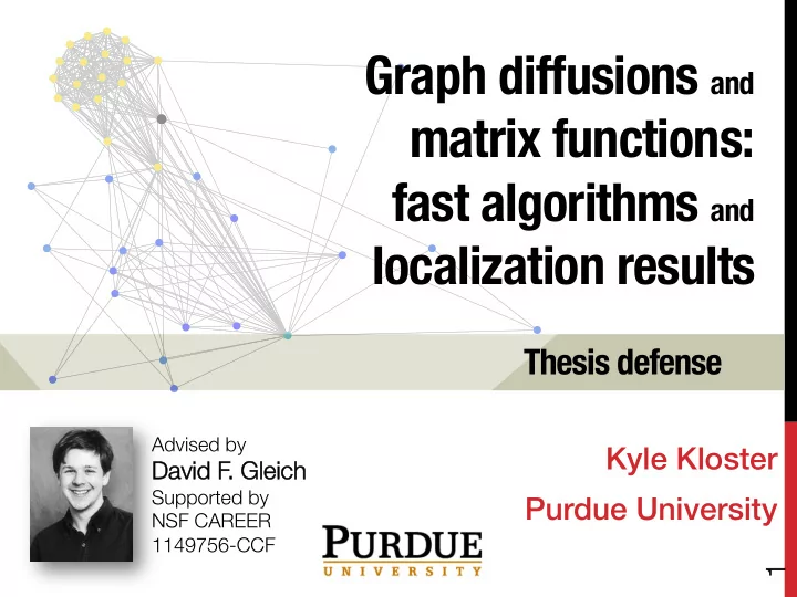
� Graph diffusions and � matrix functions: � fast algorithms and � localization results Thesis defense Advised by Kyle Kloster � David F David F. . Gleich Gleich Supported by � Purdue University � NSF CAREER 1149756-CCF 1

Network Analysis Erd ő s Number Graphs can model everything! Facebook friends Twitter followers Graph, G Search engines Amazon/Netflix rec. V , nodes Protein interactions E , edges Power grids Google Maps Air traffic control Sports rankings Cell tower placement Scheduling Parallel programming Everything 2 Kevin Bacon

� Network Analysis Recommending facebook friends Each node is a user, the graph has edges between facebook friends. � How should Facebook determine which users to recommend as new friends to the node colored black? 3

� Network Analysis PageRank One of the best methods for determining FB friends / Twitter followers is “seeded PageRank” � A diffusion process that leaks dye from target node (seed) to the rest of the graph. More dye = higher probability that node is your friend! 4

Mo’ data, mo’ problems Nonzero dye on every node (nonzero probability you are friends with each person) -> must look at whole graph to be accurate! � And real-world ~ O(10 9 ) #nodes networks are ~ O(10 10 ) #edges = |E| Big networks pose a big problem for applications that need fast answers � (like “which users should I befriend?”) 5

� � � State-of-the-art c. 2012: “Wild West” There exist “fast” methods for seeded PageRank, but they were “compute first, ask questions later”* � (or not at all!) They lacked principled mathematical theory guaranteeing these fast approximations would be accurate . � But fast approximate methods “seemed to work” 6

� Localization in seeded PageRank Newman’s In connected graphs netscience graph seeded PageRank is non-zero everywhere. � 379 vertices 924 edges But in practice… x is “zero” on most of the nodes! Seed Seed 7

Solution to Big Data: localization Local algorithms look at just the graph region near the nodes of interest Localization occurs when a global object can be approximated accurately by being precise in only a small region 8

� Weak and strong localization Weak localization: an approximation that � is sparse, and accurate enough to use in � applications that tolerate low accuracy � (clustering!) � Strong localization: an approximation that � is sparse, and accurate enough for use in any � application. 9

� � State of the art, 2016/4/22 Weak Strong localization localization PR [Nassar, K., Gleich, 2015] HK [K. & Gleich 2014] [Gleich & K., 2014] Gen � In preparation! Diff ? 10 10

Weak localization in diffusions 11 11

General diffusions: intuition A diffusion propagates “rank” from a seed across a graph. = high � seed diffusion value � = low � 12 12

Graph Matrices Adjacency matrix, A 1, if node i links to node j A ij = 0 otherwise Random-walk transition matrix, P P ij = A ji / d j d j where is the outdegree of node j. P = A T D − 1 where is the diag degree matrix. D Column stochastic! i.e. column-sums = 1 13 13

General diffusions: intuition A diffusion propagates “rank” from a seed across a graph. seed General diffusion vector c k P k ˆ X s = f ( P )ˆ f = s k =0 f = + … + p 3 p 0 + p 1 + p 2 c 3 c 0 c 1 c 2 14 14

Local Community Detection Given seed(s) S in G , find a community that contains S . seed “Community” ? high internal, low external connectivity � 15 15

Low-conductance sets are communities cut( T ) conductance( T ) = min( vol( T ), vol( T c ) ) ~ “ chance a random edge touching T also exits T ” conductance(comm) = 39/381 = .102 16 16

Graph diffusions find low-conductance sets seed = high � diffusion value � = low � = local community / � low-conductance set � 17 17

Use a diffusion for good conductance sets f ) k ∞  ε , f ≥ ˆ k D − 1 ( f � ˆ 1. Approximate f so f ≥ 0 2. Then “sweep” for best conductance set. Sweep: 1. Sort diffusion vector so f 1 / d (1) ≥ f 2 / d (2) ≥ · · · 2. Consider the sweep sets S(j) = {1,2,…,j} 3. Return the set S(j) with the best conductance. 18 18

� Weak localization in diffusions f ) k ∞  ε , f ≥ ˆ 1. Approximate f so k D − 1 ( f � ˆ f ≥ 0 Weak localization: When an approximation of f satisfies � k D − 1 ( f � ˆ and is sparse, the diffusion � f ) k ∞  ε is weakly localized. � Basically: “get just the biggest entries sort of correct” � 19 19

� � Diffusions used for conductance ∞ α k P k ˜ Personalized PageRank (PPR) � X f = s k =0 ∞ k ! P k ˜ Heat Kernel (HK) � t k X f = s k =0 Various diffusions Time-dependent PageRank (TDPR) � explore different aspects of graphs. 20 20

Diffusions: conductance & algorithms good fast conductance algorithm Local Cheeger Inequality � [Andersen Chung Lang 06] PR [Andersen,Chung,Lang 06] “PPR-push” is O(1/( ε (1- 𝛽 ))) Local Cheeger Inequality [K., Gleich ’14] HK [Chung ’07] “HK-push” is O(e t C/ ε ) [Avron, Horesh ’15] TDPR Open question Constant-time heuristically In preparation with Gleich Gen � [Ghosh et al. ’14] on L; � and Simpson Diff open question for general f 21 21

� Our algorithms for ˆ f ≈ f ( P )ˆ s - constant time on any graph, O( e 1 ˜ - heat kernel: � ε ) - general: O( N 2 ε ) k D − 1 ( f � ˆ - accuracy: f ) k ∞  ✏ - our experiments show heat kernel outperforms PageRank on real-world communities 22 22

General diffusion: Algorithm Intuition From parameters c k , ε , seed s … � Starting from here… seed seed p 3 … “residual staging area”: p 0 p 1 p 2 How to end up here? + p 3 + … + p 0 + p 1 p 2 c 3 c 1 c 2 c 0 c k P k ˆ X s = f ( P )ˆ f = s k =0 23 23

General diffusion: Algorithm Intuition     p 0 s   I p 1 0 − P I           p 2 0   − P I     =   . .       . . − P I     . .         ... ...  .   .  . . . . + p 3 + … + p 0 + p 1 p 2 c 3 c 1 c 2 c 0 c k P k ˆ X s = f ( P )ˆ f = s k =0 24 24

Algorithm Intuition Begin with mass at seed(s) seed seed in a “residual” staging area, r 0 r 3 … r 0 r 1 r 2 The residuals r k hold mass that is unprocessed – it’s like error Idea : “push” any entry r k (j)/ d j > (some threshold) + p 3 + … p 0 + p 1 + p 2 c 3 c 1 c 2 c 0 25 25

Thresholds entries < threshold ERROR equals weighted sum of entries left in the vectors r k r 3 … r 0 r 1 r 2 à Set threshold so “leftovers” sum to < ε Threshold for stage r k is � 0 1 ∞ X ε / c j @ A + p 3 + … p 0 + p 1 + p 2 c 3 c 1 c 2 c 0 j = k +1 Then k D − 1 ( f � ˆ f ) k ∞  ε 26 26

General diffusions: conclusion THM : For diffusion coefficients c k >= 0 satisfying N ∞ “rate of X and X c k = 1 c k ≤ ✏ / 2 decay” k =0 k =0 Our algorithm approximates the diffusion f k D − 1 ( f � ˆ on an undirected graph so that f ) k ∞  ✏ in work bounded by O (2 N 2 / ✏ ) Constant for any inputs! (If diffusion decays fast) 27 27

Proof sketch N X 1. Stop pushing after N terms. c k ≤ ✏ / 2 k =0 2. Push residual entries in first N terms if r k ( j ) ≥ d ( j ) ✏ / (2 N ) m k m k N − 1 N − 1 3. Total work is # pushes: X X X X r k ( j t )(2 N ) / ✏ d ( j t ) ≤ t =1 k =0 t =1 k =0 m k 4. Each r k sums to <= 1 X r k ( j t ) ≤ 1 (each push is added to f , which sums to 1) t =1 O (2 N 2 / ✏ ) 28 28

Strong localization in seeded PageRank 29 29

� � Strong localization in seeded PageRank Given a seed and a graph P = A T D − 1 e s Seeded PageRank is defined as the solution to � ( � − α P ) x = (1 − α ) e s where is the “teleportation α parameter” in (0,1). Strong localization: if we can approximate x so that � k x � ˆ x k 1  ε and the approximation is sparse, x is strongly localized. 30 30

An example on a bigger graph Crawl of flickr from 2006: ~800K nodes, 6M edges, � seeded PageRank with = 0.5 α 0 0 1.5 10 10 || x true – x nnz || 1 − 5 − 5 1 10 10 error 0.5 − 10 − 10 10 10 0 − 15 − 15 10 10 0 2 4 6 8 10 0 0 2 2 4 4 6 6 10 10 10 10 10 10 10 10 5 plot( x ) nonzeros x 10 X-axis: node index Y-axis: value at that index in true PageRank vector 31 31

� Conditions for localization? When is localization in diffusions possible? We’ve observed localization in real world graphs. Does it always occur? Are there graphs in which no localization occurs? If localization occurs *everywhere* then our result is less meaningful... 32 32

Strong localization can be impossible Consider a star graph 1 1 + α α (1 + α )( n − 1) Values in the PageRank vector seeded on the center node. Essentially everything is needed to be non-zero to get a global error bound. 33 33