Gorman-Lancaster Approach to Estimating Demand for New Good Gorman - PowerPoint PPT Presentation

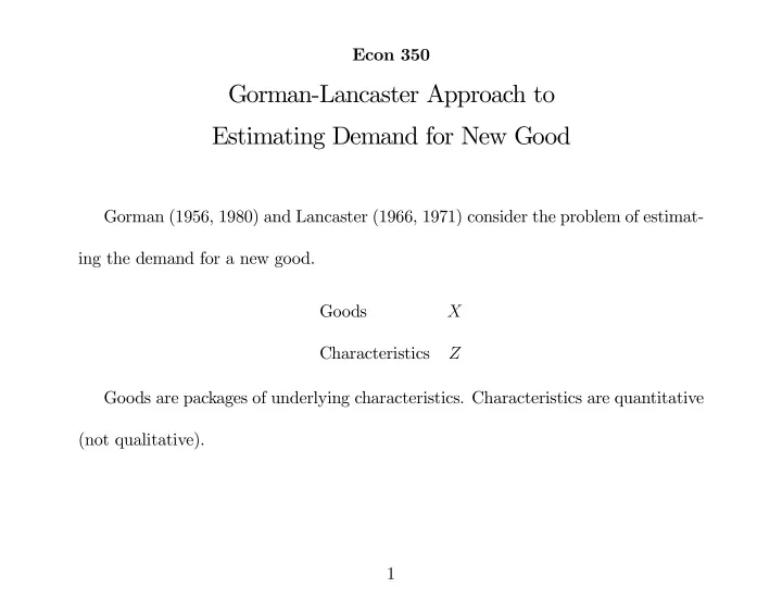
Econ 350 Gorman-Lancaster Approach to Estimating Demand for New Good Gorman (1956, 1980) and Lancaster (1966, 1971) consider the problem of estimat- ing the demand for a new good. Goods X Characteristics Z Goods are packages of underlying characteristics. Characteristics are quantitative (not qualitative). 1

Let b ij be the quantity of the i th characteristic possessed by the j th good Linearity: Z i = b ij X j ( Z i from j ) Additivity: Z i = b ij X j + b ik X k ( Z i from j and k ) Z i = P n j =1 b ij X j i = 1 , . . . , r ( Z i from all sources) r characteristics, n goods. Z = BX B is r × n . Traditional model of consumer demand assumes B is a square matrix and invertible, X = B − 1 Z. 2

General case has no such restriction. General problem: Assume U ( Z ) U is quasiconcave in Z PX ≤ M Budget constraint in goods space ⎧ ⎪ ⎪ ⎨ Z = BX ; X ≥ 0 , P > 0 max U ( Z ) such that ⎪ ⎪ ⎩ PX ≤ M Direct substitution: max U ( BX ) such that PX ≤ M leads to corner solutions and ß ats. Need a more systematic approach. 3

Budget set in goods space { X | PX ≤ M, X ≥ 0 } convex set, P > 0 . Budget set in characteristics space K = { Z | Z = BX, PX ≤ M, X ≥ 0 } feasible set. Set convex. Both sets characterized by extreme points. For goods space these are (i) the origin (0 , . . . , 0) (ii) M , . . . , M P 1 P n 4

Let X s be extreme points of goods space, s = 1 , . . . , n . Mapped by Z s = BX s to extreme points in characteristics space. µ M ¶ Z s i = b is for coordinate i P s µ M ¶ Z s = B s over all coordinates P s Budget set in characteristics space: 1. A convex polytope (convex combinations of extreme points) 2. Has at most n + 1 extreme points 3. Every extreme point in characteristics space is an extreme point in goods space. 4. An extreme point in goods space is not necessarily an extreme point in charac- teristics space. 5

X 3 M Z 2 - P 3 X 2 M M - - P 1 P 2 O Z 1 X 1 Figure 1: Case with r = 2 , n = 3 . Good 1 intensive in Z 2 : b 11 < b 12 < b 13 . b 21 b 22 b 23 6

Two-stage maximization: 1. Compute minimal cost bundles of Z . 2. Maximize utility in Z space. Implications: no longer have a representative agent, except under extreme condi- tions. 7

X 3 Z 2 M - P 3 X 2 M M - - P 2 P 1 O Z 1 X 1 Figure 2: Case with r = 2 , n = 3 , with b 11 < b 12 < b 13 . b 21 b 22 b 23 8

Problem has two aspects: 1. De Þ ne Goods E ffi ciency Set 2. Maximize over Goods E ffi ciency Set Maximize U ( Z ) such that Z ∈ K. (a) Every point on the e ffi ciency frontier in C space is the image of a point on budget in goods space. (b) A point on e ffi ciency frontier in goods space not necessarily on e ffi ciency frontier in characteristics space (see above). 9

Vertex Optima Z 2 Facet Optima O Z 1 Figure 3: Indi ff erence Curves. 10

Concept: E ffi ciency Frontier 1. As income expands, polytope expands proportionately. 2. As price of good 2 increases, it is less likely to be bought. 3. At a su ffi ciently high price, the good drops out. Two e ff ects: 1. E ffi ciency Substitution E ff ect 2. Personal Substitution E ff ect Can get inferior goods even if all characteristics are normal. ∴ Normal in Characteristics. Not in goods. 11

Z 2 Good 2 Good 1 Price at which consumers are indifferent between 1 and 3 Drops out of choice set Good 3 O Z 1 Figure 4: E ffi ciency Frontier with b 11 < b 12 < b 13 . b 21 b 22 b 23 12

Return to the stated problem: how to estimate the demand for a new good? Recall Knight’s Quotation. Need to make the future like the past. Lancaster Approach: 1. Assume a common technology B across all consumers. 2. Need a model of preferences. 3. Why are people who are observationally identical buying di ff erent goods? (Model of Preference Heterogeneity) 13

Consider the following example: 1. We observe X, Z 2. ∴ We can identify B 3. Estimate Preferences U ( Z ) allowing for heterogeneity in preferences (no more representative consumer). 4. Forecast demand for new good as a vector of characteristics. 14

Is Good 3 purchased? NO Is Good 3 0 purchased? YES ∴ We estimate the technology of purchase or not (purely a technical a ff air). 15

Z 2 (3 ' ) (1) (3) not purchased (2) O Z 1 Figure 5: Example with n = r = 2 . Goods (1) and (2) are in the choice set. 16

Consider a case where only (1) and (2) are bought (and maybe only (1) or (2)). ⎛ ⎞ ⎜ b 11 b 12 ⎟ Assume B is nonsingular. ⎜ ⎟ B = ⎝ ⎠ b 21 b 22 Rows: characteristics; Columns: goods b 11 < b 12 (as drawn) b 21 b 22 Good 2 intensive in Z 1 . Good 1 intensive in Z 2 . Need to know distribution of preferences. Take the Two Good World, n = r = 2 . 17

Example: 1 Z 1 − α U = Z α , 0 ≤ α ≤ 1 2 Distribution of Income M F M ( M ) Distribution of α F α ( α ) Consumer buys both goods if on (1)—(2) face. µ ¶ Z 2 α = P Z 1 1 − α Z 1 P Z 2 18

Z 2 (3 ' ) (1) (2) 2 O Z 1 Figure 6: Case where all three are bought. 19

Cobb-Douglas Þ xes shares: µ ¶ µ ¶ α = P Z 1 Z 1 α so ( P Z 2 Z 2 ) = P Z 1 Z 1 1 − α P Z 2 Z 2 1 − α P Z 2 Z 2 + P Z 1 Z 1 = M P Z 2 Z 2 = (1 − α ) M P Z 1 Z 1 = αM Z 2 = (1 − α ) M Z 1 = α M , P Z 2 P Z 1 20

Buy good 1 only if we have µ ¶ µ b 21 ¶ α ≥ P Z 1 . 1 − α b 11 P Z 2 In general, b 22 ≤ Z 2 ≤ b 21 . b 12 Z 1 b 11 21

Therefore, we have three types of solutions: buy good 1 only, buy good 2 only or buy both. α Map α − → 1 − α = V, F V ( V ) is cdf. Assume it has density f V ( V ) (absolutely continuous with respect to Lebesgue mea- sure), ⎛ ⎞ µ µ P Z 1 ¶ b 12 ¶ good 2 bought ⎜ ⎟ ⎜ ⎟ Pr = Pr V ≤ , ⎝ ⎠ P Z 2 b 22 exclusively ⎛ ⎞ µ µ P Z 1 ¶ b 11 ¶ good 1 bought ⎜ ⎟ ⎜ ⎟ Pr = Pr V ≥ . ⎝ ⎠ P Z 2 b 21 exclusively 22

Mixed Discrete-Continuous Model. α M Z 1 = P Z 1 (1 − α ) M Z 2 = P Z 2 Given the distribution of ( α, M ) , can derive demands. Goal of Structural Estimation: to identify F α or F V . For example, if V ∼ λe − λV = f V ( V ) , µ µ P Z 1 ¶¶ Z PZ 1 b 11 b 11 PZ 2 b 21 λe − λV dV = exp Pr ( good 2 bought ) = − λ . P Z 2 b 21 0 23

Can identify λ from ³ ´ \ ln Pr ( good 2 bought ) = ˆ µ P Z 1 ¶ µ b 11 ¶ − λ P Z 2 b 21 where b denotes estimate. 24

Can recover F α . How? Trivial: ⎛ ¯ ⎞ ¯ P Z 1 b 11 P Z 1 b 12 ¯ ⎜ ¯ ⎟ P Z 2 b 21 P Z 2 b 22 ⎜ ¯ ⎟ g ⎝ α ≤ α ≤ ¯ ⎠ 1 + P Z 1 b 12 1 + P Z 1 b 12 ¯ ¯ P Z 2 b 22 P Z 2 b 22 ¯ µ ¶ ¯ P Z 1 b 11 1 − α ≤ P Z 1 α b 12 ¯ = g α ≤ , ¯ P Z 2 b 21 P Z 2 b 22 α i.e. if we know the distribution of a < 1 − α < b , we know the distribution of a b a + 1 ≤ α ≤ b + 1 . 25

In this technology, if B − 1 exists Z = BX B − 1 Z = X PB − 1 Z = PX = M ¡ PB − 1 ¢ = P Z . µ b 13 ¶ If we introduce a good with intensity , who buys it? And in what amounts? b 23 26

Suppose b 22 ≤ b 23 ≤ b 21 . b 12 b 13 b 11 Per unit cost of Z 1 from good 3 is P 3 . Per unit cost of Z 2 from good 3 is P 3 if b 13 b 23 ⎛ ⎞ P 3 ⎜ ⎟ b 13 ⎜ ⎟ ⎠ ≥ PB − 1 . ⎝ P 3 b 23 Good drops out of the budget. 27

Breakeven Price Z 2 (3) (1) (2) O Z 1 Figure 7: People buy good if b 22 ≤ b 23 ≤ b 21 . b 12 b 13 b 11 28