GENETIC ALGORITHMS: PREREQUISITES Date: Friday 18 March 2016 - PowerPoint PPT Presentation

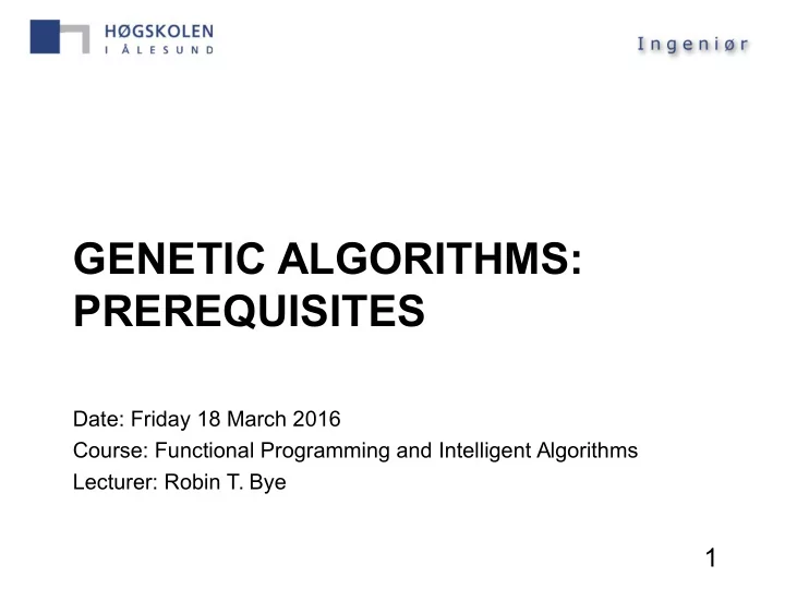
GENETIC ALGORITHMS: PREREQUISITES Date: Friday 18 March 2016 Course: Functional Programming and Intelligent Algorithms Lecturer: Robin T. Bye 1

Topics in this module • Introduction to AI and optimisation • Nature-inspired algorithms – Focus on the genetic algorithm (GA) • Binary GAs • Continuous GAs • Basic applications • Real-life case study 2

Recommended reading • Main text: Practical Genetic Algorithms , Haupt and Haupt, 2nd Ed., 2004. • Supplementary texts: – Machine Learning: An Algorithmic Perspective , Marsland, 2nd Ed., 2015. – Artificial Intelligence: A Guide to Intelligent Systems , Negnevitsky, 2nd Ed., 2002. – Genetic Algorithms in Search, Optimization and Machine Learning , Goldberg, 1989. – Artificial Intelligence: A Modern Approach , Russell and Norvig, 3rd Ed., 2010. 3

Introduction to artificial intelligence (AI) 4

What is AI? • Many definitions exist • Russell and Norvig (R&N): «The study and design of intelligent agents» – But what is an intelligent agent? • Intelligent agent (R&N): «a system that perceives its environment and takes actions that maximize its chances of success» 5

What is AI? • AI is a huge field involved with topics such as – Problem-solving – Knowledge, reasoning, planning – Uncertain knowledge and reasoning – Learning – Communicating, perceiving, acting (categories from R&N) 6

Tools in AI • Search and optimisation – Useful in problem-solving • Logic • Probabilistic methods • Classifiers and statistical learning • Neural networks • Control theory • Languages 7

Engineering is problem-solving • Engineering is about solving real-world problems • Many tools available, particularly search and optimisation • Heuristic methods useful, e.g. genetic algorithms 8

Some real-world problems • Routing video streams in network • Airline travel-planning system • Traveling salesperson problem (TSP) • VLSI layout problem • Robot navigation • Automatic assembly sequencing • ... And million others 9

Introduction to optimisation 10

What is optimisation? • A process of improving an existing idea • Goal: Finding the best solution – What does”best” mean? • With exact answers, ”best” may have a specific definition, eg., PL top scorer • Other times, best is a relative definition, eg., prettiest actress or best lecturer 11

What is optimisation? • A process of adjusting inputs to a system to find max/min output • Inputs: Variables, e.g., x, y, z • System: Cost function, e.g., f(x,y,z) • Output: Cost evaluated at particular values of variables, e.g., C=f(x0,y0,z0) • Search space: Set of possible inputs, eg. all possible values of x, y, z 12

What is optimisation? Inputs System (function) Output (cost) x y f(.) C=f(x,y,z) z Q: What are the dimensions of the search space? • Challenge: Determine optimal inputs x*,y*,z* that C=f(x) minimises cost C. • 1D example: C min = f(x*) x* x C min 13

Note on convention • Optimisation is to find the minimum cost • Equivalently, maximise fitness • Cost function = (minus) fitness function • Maximisation is the same as minimising the negative of the cost function (put minus in front) • Maximising 1-x^2  minimising x^2-1 14

Root finding vs. optimisation • Root finding: Searches for the zero of a function • Optimisation: Searches for the zero of the function derivative • 2nd derivative to determine if min/max • Challenge: Is minimum global (optimal) or local (suboptimal)? 15

Categories of optimisation • Trial and error vs. function • Single- vs. multivariable • Static vs. dynamic • Discrete vs. continuous • Constrained vs. unconstrained • Random vs. minimum seeking 16

Trial and error vs. function • Trial and error method: Adjust variables/inputs without knowing how the output will change  experimentalist approach • Function method: Known cost function, thus may search variables/inputs in clever ways to obtain desired (optimal) output  theoretician approach 17

Single- vs. multivariable • Single variable: One-dimensional (1D) optimisation • Multivariable: Multi-dimensional (nD) optimisation – Difficulty increases with dimension number • Sometimes can split up nD optimisation in n series of 1D optimisations 18

Dynamic vs. static • Dynamic: Output is a function of time (optimal solution changes with time) • Static: Output is independent of time (finding optimal solution once is enough) • Example: Shortest distance from A to B in a city is static, but fastest route depends on traffic, weather, etc. at a given time 19

Discrete vs. continuous • Discrete: Finite number of variable values – Known as combinatorial optimisation – Eg. optimal order to do a set of tasks • Continuous: Variables have infinite number of possible values – Eg. f(x) = x^2 20

Constrained vs. unconstrained • Constrained: Variables confined to some range – eg., –1 < x < 1 • Unconstrained: Any variable value is allowed, eg., x is a real number 21

Minimum-seeking vs. random • Minimum-seeking: Derivative method going downhill until reached minimum – Fast – May get stuck at local minimum • Random: Probabilistic method – Slower – Better at finding global minimum 22

Minimum-seeking algorithms 23

Cost surface • Cost surface consists of all possible function values • 2D case: All values of f(x,y) make up the cost surface (height = cost) • Goal: Find minimum cost (height) in cost surface • Downhill strategy  easily stuck in local minimum • Can be multi-dimensional 24

Exhaustive search • Brute force approach: Divide cost surface into large number of sample points. • Check (evaluate) all points • Choose variables that correspond to minimum • Computationally expensive and slow 25

Exhaustive search • Do not get stuck in local minimum • May still miss global minimum due to undersampling • Refinement: First a coarse search of large cost region, then a fine search of smaller regions 26

Analytical optimisation • Employ calculus (derivative methods) • Eg., 1D case: f(x) is continuous – Find root x_m such that derivative f’(x_m)=0 – Check 2nd derivative • if f’’(x_m) > 0, f(x_m) is minimum • if f’’(x_m) < 0, f(x_m) is maximum • Use gradient for multi-dim cases – eg., solve grad f(x,y,z) = 0 27

Analytical optimisation • Problems: – Which minimum is global? • Must search through all found minima – Requires cts. differentiable functions with analytical gradients – Difficult with many variables – Suffers at cliffs or boundaries in cost surface 28

Well-known algorithms • Nelder-Mead downhill simplex method • Optimization based on line minimisation – Coordinate search method – Steepest descent algorithm – Newton’s method techniques – Quadratic programming • Natural optimisation methods 29