Generating Loop Invariants via Polynomial Interpolation Marc Moreno - PowerPoint PPT Presentation

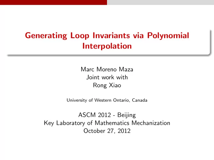
Generating Loop Invariants via Polynomial Interpolation Marc Moreno Maza Joint work with Rong Xiao University of Western Ontario, Canada ASCM 2012 - Beijing Key Laboratory of Mathematics Mechanization October 27, 2012

Plan 1 Preliminaries Notions on loop invariants Poly-geometric summations 2 Invariant ideal of P -solvable recurrences Degree estimates for solutions of P -solvable recurrences P -solvable recurrences Degree estimates for solutions of P -solvable recurrences Degree estimates for their invariant ideal Dimension estimates for their invariant ideal 3 Loop invariant generation via polynomial interpolation A direct approach A modular method Maple Package: ProgramAnalysis

Preliminaries Notions on loop invariants Plan 1 Preliminaries Notions on loop invariants Poly-geometric summations 2 Invariant ideal of P -solvable recurrences Degree estimates for solutions of P -solvable recurrences P -solvable recurrences Degree estimates for solutions of P -solvable recurrences Degree estimates for their invariant ideal Dimension estimates for their invariant ideal 3 Loop invariant generation via polynomial interpolation A direct approach A modular method Maple Package: ProgramAnalysis

Preliminaries Notions on loop invariants Loop model under study while C 0 do if C 1 then 1 Loop variables: X = x 1 , . . . , x s , X := A 1 ( X ) ; rational value scalar elif C 2 2 Conditions: each C i is a quantifier free then formula in X over Q . X := A 2 ( X ) ; 3 Assignments: A i ∈ Q [ X ] inducing a · · · polynomial map M i : R s �→ R s elif C m then 4 Initial condition: X -values defined by a X := A m ( X ) ; semi-algebraic system. end if end while

Preliminaries Notions on loop invariants Basic notions x, y, a, b are loop variables since they are updated in the loop or used to update other x := a ; loop variables. y := b ; The set of the initial values of the loop is while x < 10 do x := x + y 5 ; { ( x, y, a, b ) | x = a, y = b, ( a, b ) ∈ R 2 } . y := y + 1 ; The loop trajectory of the above loop starting end do; at ( x, y, a, b ) = (1 , 0 , 1 , 0) is the sequence: (1 , 0 , 1 , 0) , (1 , 1 , 1 , 0) , (2 , 2 , 1 , 0) , (34 , 3 , 1 , 0) . The reachable set R ( L ) of a loop L consists of all tuples of all trajectories of L . If x 1 , . . . , x s are the loop variables of L , then a polynomial P ∈ Q [ x 1 , . . . , x s ] is a (plain) loop invariant of L whenever R ( L ) ⊆ V ( P ) holds.

Preliminaries Notions on loop invariants More notions The inductive reachable set R ind ( L ) of a loop L is the reachable set of the loop obtained from L by replacing the guard condition with true. The absolute reachable set R abs ( L ) of a loop L is the reachable set of the loop obtained from L by replacing the guard condition with true, ignoring the branch conditions and, at each iteration executing a branch action selected randomly. We clearly have R ( L ) ⊆ R ind ⊆ R abs

Preliminaries Notions on loop invariants More notions The inductive reachable set R ind ( L ) of a loop L is the reachable set of the loop obtained from L by replacing the guard condition with true. The absolute reachable set R abs ( L ) of a loop L is the reachable set of the loop obtained from L by replacing the guard condition with true, ignoring the branch conditions and, at each iteration executing a branch action selected randomly. We clearly have R ( L ) ⊆ R ind ⊆ R abs If x 1 , . . . , x s are the loop variables of L , then a polynomial P ∈ Q [ x 1 , . . . , x s ] is an inductive (resp. absolute) loop invariant of L whenever R ind ( L ) ⊆ V ( P ) (resp. R abs ( L ) ⊆ V ( P ) ) holds. We denote by I ( L ) (resp. I ind ( L ) , I abs ( L ) ) the set of the polynomials that are plain (resp. inductive, absolute) loop invariants of L . These are radical ideals such that I abs ( L ) ⊆ I ind ( L ) ⊆ I ( L )

Preliminaries Notions on loop invariants Absolute invariants might be trivial Consider y 1 x 2 + y 2 + y 3 = x 1 ( E ) . y 1 := 0 ; If x 1 = 0 then the equation ( E ) holds initially y 2 := 0 ; and the loop is not entered. y 3 := x 1 ; If x 1 � = 0 and x 2 = 1 then ( E ) and while y 3 � = 0 do y 2 + 1 = x 2 hold before each iteration. if y 2 + 1 = x 2 If x 1 � = 0 and x 2 � = 1 then the second action then preserves ( E ) . y 1 := y 1 + 1 ; y 2 := 0 ; Therefore y 1 x 2 + y 2 + y 3 − x 1 ∈ I ( L ) and y 3 := y 3 − 1 ; y 1 x 2 + y 2 + y 3 − x 1 ∈ I ind ( L ) both hold. else y 2 := y 2 + 1 ; y 3 := y 3 − 1 ; end if end do

Preliminaries Notions on loop invariants Absolute invariants might be trivial Consider y 1 x 2 + y 2 + y 3 = x 1 ( E ) . y 1 := 0 ; If x 1 = 0 then the equation ( E ) holds initially y 2 := 0 ; and the loop is not entered. y 3 := x 1 ; If x 1 � = 0 and x 2 = 1 then ( E ) and while y 3 � = 0 do y 2 + 1 = x 2 hold before each iteration. if y 2 + 1 = x 2 If x 1 � = 0 and x 2 � = 1 then the second action then preserves ( E ) . y 1 := y 1 + 1 ; y 2 := 0 ; Therefore y 1 x 2 + y 2 + y 3 − x 1 ∈ I ( L ) and y 3 := y 3 − 1 ; y 1 x 2 + y 2 + y 3 − x 1 ∈ I ind ( L ) both hold. else If conditions are ignored, ( x 1 , x 2 ) = (0 , 1) and y 2 := y 2 + 1 ; execute the first branch once, then we obtain y 3 := y 3 − 1 ; y 1 x 2 = 1 and y 2 + y 3 = x 1 . end if end do Then ( E ) is violated and we have I abs ( L ) = � 0 � .

Preliminaries Notions on loop invariants Inductive invariants might not be plain invariants x := 1 ; x − 1 = 0 is an invariant but not an inductive while x � = 1 do of the following loop. x := x + 1 ; Thus I ind ( L ) is strictly smaller than I ( L ) end do

Preliminaries Notions on loop invariants Computing inductive invariants via elimination ideals Solving for ( x, y ) as a 2-variable recurrence x ( n + 1) = y ( n ) , y ( n + 1) = x ( n ) + y ( n ) , with x (0) = 0 , y (0) = 1 . We obtain y := 1 ; √ √ 5+1 5+1 ) n ) n ( ( − x := 0 ; x ( n ) = − , √ 2 √ 2 5 5 while true do √ √ √ √ 5+1 5+1 ) n ) n ( ( − 5+1 − − 5+1 y ( n ) = . √ 2 √ 2 z := x ; 2 2 5 5 √ √ √ x := y ; 5+1 ) n , v = ( − 5+1 ) n , a = Let u = ( 5 2 2 y := z + y ; Taking the dependencies u 2 v 2 = 1 , a 2 = 5 into end while account, we want 5 , a 2 − 5 , y − a a +1 5 + a − a +1 � x − au 5 + av u v 2 2 5 , u 2 v 2 − 1 � ∩ Q [ x, y ] , which is � 1 − y 4 + 2 xy 3 + x 2 y 2 − 2 x 3 y − x 4 � .

Preliminaries Notions on loop invariants Summary and notes Computing I ind ( L ) is a better approximation of I ( L ) than I abs ( L ) . The loop invariant generation methods of (E. Rodriguez-Carbonell & D. Kapur, ISSAC04) and (L. Kov´ acs, TACAS08) focus on I abs ( L ) .

Preliminaries Notions on loop invariants Summary and notes Computing I ind ( L ) is a better approximation of I ( L ) than I abs ( L ) . The loop invariant generation methods of (E. Rodriguez-Carbonell & D. Kapur, ISSAC04) and (L. Kov´ acs, TACAS08) focus on I abs ( L ) . In this talk, we target I ind ( L ) (easier to compute than I ( L ) ) and call it the Invariant Ideal of the loop L . Same goal as in (Bin Wu, Liyong Shen, Min Wu, Zhengfeng Yang & Zhenbing Zeng, 2011).

Preliminaries Notions on loop invariants Summary and notes Computing I ind ( L ) is a better approximation of I ( L ) than I abs ( L ) . The loop invariant generation methods of (E. Rodriguez-Carbonell & D. Kapur, ISSAC04) and (L. Kov´ acs, TACAS08) focus on I abs ( L ) . In this talk, we target I ind ( L ) (easier to compute than I ( L ) ) and call it the Invariant Ideal of the loop L . Same goal as in (Bin Wu, Liyong Shen, Min Wu, Zhengfeng Yang & Zhenbing Zeng, 2011). We also want to avoid computing closed forms of loop variables, while • not making any assumptions on the shape of the polynomial invariants, • and avoiding an intensive use of expensive algebraic computations other than linear algebra, for which costs are predictable.

Preliminaries Notions on loop invariants Summary and notes Computing I ind ( L ) is a better approximation of I ( L ) than I abs ( L ) . The loop invariant generation methods of (E. Rodriguez-Carbonell & D. Kapur, ISSAC04) and (L. Kov´ acs, TACAS08) focus on I abs ( L ) . In this talk, we target I ind ( L ) (easier to compute than I ( L ) ) and call it the Invariant Ideal of the loop L . Same goal as in (Bin Wu, Liyong Shen, Min Wu, Zhengfeng Yang & Zhenbing Zeng, 2011). We also want to avoid computing closed forms of loop variables, while • not making any assumptions on the shape of the polynomial invariants, • and avoiding an intensive use of expensive algebraic computations other than linear algebra, for which costs are predictable. In (Sankaranarayanan, Sipma & Manna, SIGPLAN 2004) (Y. Chen, B. Xia, L. Yang, & N. Zhan, FMHRTS 2007) (D. Kapur Deduction and Applications 2005) template polynomials are used. Moreover, the latter two use real QE.