Generating and Solving Symbolic Parity Games Gijs Kant Jaco van de - PowerPoint PPT Presentation
Generating and Solving Symbolic Parity Games Gijs Kant Jaco van de Pol Formal Methods & Tools University of Twente The Netherlands Games 2012, Napoli, Italia 1 / 26 Motivation Application: formal verification of process algebraic
Generating and Solving Symbolic Parity Games Gijs Kant Jaco van de Pol Formal Methods & Tools University of Twente The Netherlands Games 2012, Napoli, Italia 1 / 26
Motivation ◮ Application: formal verification of process algebraic specifications ◮ Process algebra mCRL2: behaviour of a system P ◮ First-order modal µ -calculus formula ϕ : desired property of the system ◮ P | = ϕ is translated to a first-order boolean equation system ◮ An appropriate way to solve such a system is by instantiation to a parity game ◮ These parity games, however, can become rather large 2 / 26
Contents Practical solving of first-order boolean equation systems using symbolic data structures. ◮ Translation from process algebra and µ -calculus to first-order boolean equations ◮ Instantiation from first-order boolean equation system to a parity game . . . using LTSmin : symbolic generation (using MDDs) ◮ Symbolic solving using spgsolver . ◮ Two case studies 3 / 26
mCRL2 ◮ mCRL2 language ( mcrl2.org ): algebraic data types, parallel composition, etc. ◮ Several analysis techniques: simulation, visualisation, model checking. ◮ Linear Process Specification (LPS) format: summands of the � form guard → action . recursion d : D Example proc Buffer ( q : List ( D )) = � (# q < 2 ) → read ( d ) . Buffer ( q ⊳ d ) d : D + ( q � = []) → send ( head ( q )) . Buffer ( tail ( q )); init Buffer ([]); 4 / 26
First-order Boolean Equation System Definition A first-order boolean equation system (or parameterised boolean equation system ) is a system of equations with boolean variables that can have data parameters and has boolean expressions that can have quantifiers and operators over arbitrary data types. 5 / 26
lps2pbes proc Buffer ( q : List ( D )) = � (# q < 2 ) → read ( d ) . Buffer ( q ⊳ d ) d : D + ( q � = []) → send ( head ( q )) . Buffer ( tail ( q )); init Buffer ([]); Deadlock freedom: infinitely often after any action ( [ ⊤ ] X ), always some action is enabled ( �⊤� ⊤ ): ν X . �⊤� ⊤ ∧ [ ⊤ ] X translates for the simple buffer to: pbes ν X ( q : List ( D )) = ( q � = []) ∨ (# q < 2 ) ∧ ∀ d ∈ D . (# q < 2 ) ⇒ X ( q ⊳ d ); ∧ ( q � = []) ⇒ X ( tail ( q )) init X ([]); 6 / 26
Instantiation pbes ν X ( q : List ( D )) = ( q � = []) ∨ (# q < 2 ) ∧ ∀ d ∈ D . (# q < 2 ) ⇒ X ( q ⊳ d ); ∧ ( q � = []) ⇒ X ( tail ( q )) init X ([]); This system of equations instantiates to: µ X ([]) = true ∧ X ([ d 1 ]) ∧ X ([ d 2 ]) µ X ([ d 1 ]) = true ∧ X ([ d 1 , d 1 ]) ∧ X ([ d 1 , d 2 ]) ∧ X ([]) µ X ([ d 2 ]) = . . . µ X ([ d 1 , d 1 ]) = . . . µ X ([ d 1 , d 2 ]) = . . . which can be seen as a two-player game. 7 / 26
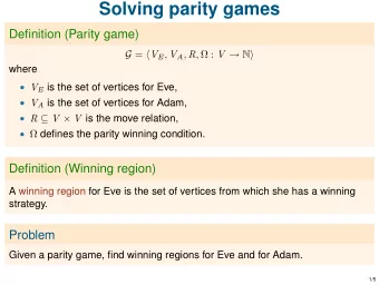
Parity Games Definition (Parity Game) A parity game is a graph G = � V , E , V 0 , V 1 , v I , Ω � , with ◮ V the finite set of vertices (or places or states); ◮ E : V × V the set of transitions; ◮ V 0 ⊆ V the set of places owned by player 0 ; ◮ V 1 ⊆ V the set of places owned by player 1 ; ◮ v I ∈ V the initial state of the game; ◮ Ω : V → N assigns a priority Ω( v ) to each vertex v ∈ V ; ν blocks Even priorities (0, 2, 4, . . . ) µ blocks Odd priorities (1, 3, 5, . . . ) ∨ , ∃ , �� Player 0 , ∃ loise, Even, Prover ∧ , ∀ , [] Player 1 , ∀ belard, Odd, Refuter 8 / 26
Example: Tic tac toe Example sort Player = struct X | O | − ; Board = List ( List ( Player )); pbes µ Z ( b : Board , p : Player ) = ( p = X ∧ ∃ x , y ∈ Pos . ( x ≤ 3 ∧ y ≤ 3 ) ∧ ( b [ x ][ y ] = − ) ∧ Z ( Put ( b , p , x , y ) , Opponent ( p ))) ∨ ( p = O ∧ ∀ x , y ∈ Pos . ( x ≤ 3 ∧ y ≤ 3 ) ∧ ( b [ x ][ y ] = − ) ∧ Z ( Put ( b , p , x , y ) , Opponent ( p ))) ∨ (some winning conditions for X); init Z ([[ − , − , − ] , [ − , − , − ] , [ − , − , − ]] , X ); 9 / 26
Instantiation ◮ A state Z ([[ − , − , − ] , [ − , − , − ] , [ − , − , − ]] , X ) is explored by substituting the concrete parameters for the data parameters in the formula associated with equation Z and rewriting the formula. ◮ This yields either a conjunction or disjunction of new states and possibly the boolean values true or false . ◮ For the example, rewriting the formula will yield Z ([[ X , − , − ] , [ − , − , − ] , [ − , − , − ]] , O ) ∨ Z ([[ − , X , − ] , [ − , − , − ] , [ − , − , − ]] , O ) ∨ Z ([[ − , − , X ] , [ − , − , − ] , [ − , − , − ]] , O ) ∨ . . . 10 / 26
∃ X X X . . . ∀ X X O . . . . . . . . . . . . ∃ X O . . . ∀ X X O X O . . . ∃ X O X O X O X O X X O . . . . . . X O X X O O O X O X X . . . ⊤ ⊥ 11 / 26
Instantiation ◮ Instantiating is generating a large graph and is much like state-space generation for LTSs. ◮ LTSmin : ◮ High performance verification tool. ◮ Supports multiple modelling languages. ◮ Explicit sequential, multicore and distributed generation with transition caching ◮ Symbolic generation 12 / 26
LTSmin LTSmin s view on the world: ◮ States are vectors of integers � x 0 , x 1 , · · · , x M � (other value types are stored in a database). ◮ A Next function is available that computes successor states for a state. ◮ For all kinds op optimisations, we split both state vector and next state function: ◮ the elements x i of the vector are called parts (the data parameters). ◮ the parts of the equations are called transition groups (the conjuncts/disjuncts). ◮ Independence (related to locality ): a group g is dependent on part i if the variable that is stored in slot i is read or changed by the expression of group g . 13 / 26
Dependency matrix Example pbes µ Z ( b 1 , 1 , b 1 , 2 , b 1 , 3 , b 2 , 1 , . . . , p : Player ) = ( b 1 , 1 = − ) ∧ Z ( p , b 1 , 2 , b 1 , 3 , b 2 , 1 , . . . , Opponent ( p )) ∨ (( b 1 , 2 = − ) ∧ Z ( b 1 , 1 , p , b 1 , 3 , b 2 , 1 , . . . , Opponent ( p ))) ∨ (( b 1 , 3 = − ) ∧ Z ( b 1 , 1 , b 1 , 2 , p , b 2 , 1 , . . . , Opponent ( p ))) . . . Z ( − , − , − , − , − , − , − , − , − , X ); init The matrix would then look like: g Var b 1 , 1 b 1 , 2 b 1 , 3 . . . p 1 r + – – + 2 r – + – + 3 r – – + + 4 14 / 26
Transition Groups Is a state is encoded as � 0 , 0 , 0 , 0 , 1 , 1 , 0 , 1 , 0 , 1 � and has successor � 0 , 0 , 0 , 0 , 1 , 1 , 0 , 1 , 1 , 1 � for group g , which is dependent only on vector slots 8 and 9 (the last two), i.e., in row g only cells 8 and 9 have a ‘+’ or an ‘r’. we store the computed transition as �� 0 , 1 � , � 1 , 1 �� This transition will be applied to any state matching 0 , 1 in slots 8 and 9 (we use projection of the state vector) without calling the formula rewriter. 15 / 26
Symbolic Generation Sets and relations are stored as Multivalue Decision Diagrams (MDDs), which are graph representations of a function f : Int n → Bool E.g., 3 4 1 4 1 1 2 1 3 2 2 1 3 ⊤ 16 / 26
Solving Parity Games ◮ Player 0 is the winner of a play π if min ( Inf (Ω( π ))) , the minimum of the priorities that occur infinitely often in π , is even. ◮ Player 0 is the winner of the game iff there exists a winning strategy for player 0 , i.e., from the initial state every play conforming to the strategy will be won by player 0 . ◮ Verification: player 0 is the winner of the game iff the property holds for the system. 17 / 26
Recursive algorithm (Zielonka) SolveRecursive ( G ) 1: if V = ∅ then return �∅ , ∅� 2: 3: m := min { Ω( v ) | v ∈ V } ; p := m mod 2 4: U := { v ∈ V | Ω( v ) = m } 5: A := Attr p ( G , U ) 6: � X 0 , X 1 � := SolveRecursive ( G \ A ) 7: if X 1 − p = ∅ then W p := A ∪ X p 8: W 1 − p := ∅ 9: 10: else B := Attr 1 − p ( G , X 1 − p ) 11: � Y 0 , Y 1 � := SolveRecursive ( G \ B ) 12: W p := Y p 13: W 1 − p := B ∪ Y 1 − p 14: 15: return � W 0 , W 1 � 18 / 26
Attractor Set Computation Attr p ( G , U ) 1: A := U {Result set} 2: L := U {Set of nodes added in a level} 3: while not L = ∅ do A ′ := Prev ( L ) { A ′ contains the predecessor nodes of L } 4: L := V p ∩ A ′ 5: B := Next ( A ′ ) \ A 6: B ′ := Prev ( B ) { B ′ contains the predecessor nodes of B , i.e., 7: the nodes from which the other player can choose to move to a node that is not in A .} L := L ∪ ( V 1 − p ∩ ( A ′ \ B ′ )) 8: L := L \ A 9: A := A ∪ L 10: 11: return A 19 / 26
Successor sets � Next ( V ) = Next g ( V ) 0 ≤ g < M 20 / 26
Experiments ◮ Tools are available in the development versions of mCRL2 and LTSmin . ◮ Several options for choosing the partitioning into transition groups: ◮ simple : only one group per equation ◮ split : split into conjuncts/disjuncts ◮ structured : preserve the structure of the mCRL2 model 21 / 26
Connect Four 7 × 6 board ∼ 4.5 trillion states. Whether player Yellow has a winning strategy: µ X . [ Wins ( Red )] false ∧ � Move � ( � Wins ( Yellow ) � true ∨ [ Move ] X ) 22 / 26
Recommend
More recommend
Explore More Topics
Stay informed with curated content and fresh updates.
