Generalized tensor methods and entanglement measurements for models - PowerPoint PPT Presentation
Generalized tensor methods and entanglement measurements for models with long-range interactions Ors Legeza in collaboration with Jen o S olyom, Gergely Barcza (Budapest) Florian Gebhard, Reinhard M. Noack (Marburg) Valentin
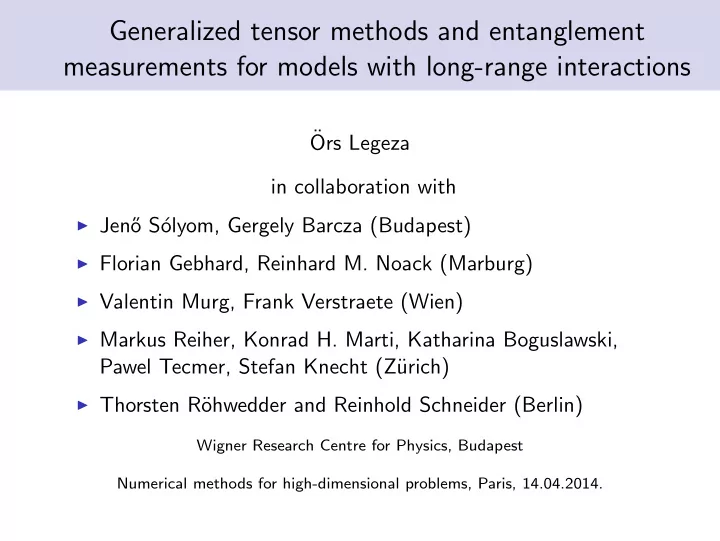
Generalized tensor methods and entanglement measurements for models with long-range interactions ¨ Ors Legeza in collaboration with ◮ Jen˝ o S´ olyom, Gergely Barcza (Budapest) ◮ Florian Gebhard, Reinhard M. Noack (Marburg) ◮ Valentin Murg, Frank Verstraete (Wien) ◮ Markus Reiher, Konrad H. Marti, Katharina Boguslawski, Pawel Tecmer, Stefan Knecht (Z¨ urich) ◮ Thorsten R¨ ohwedder and Reinhold Schneider (Berlin) Wigner Research Centre for Physics, Budapest Numerical methods for high-dimensional problems, Paris, 14.04.2014.
Brief historical overview ◮ Renormalization Group (Kadanoff transformation) (1966) ◮ Block Renormalization Group (BRG) method ◮ Numerical Renormalization Group (NRG): Wilson(1975) ◮ Density Matrix Renormalization Group (DMRG): White(1992) ◮ Quantum chemistry version of DMRG (QC-DMRG): White(1999),Mitrushenkov(2001),Chan(2002),Legeza(2002), Reiher(2005),Zgid(2006),Yanai(2008),Xiang(2010), Ma(2012), Wouters(2013)... ◮ Matrix Product State (MPS): ¨ Ostlund, Rommer(1995), Cirac, Verstraete(2004), Oseledets(2009)
Some useful reviews, also see additional references therein ◮ U. Schollw¨ ock, Rev. Mod. Phys. 77 , 259 (2005). ◮ R. M. Noack and S. R. Manmana, in Diagonalization- and Numerical Renormalization-Group-Based Methods for Interacting Quantum Systems, (AIP, 2005), vol. 789, pp. 93–163. ◮ F. Verstraete, J.I. Cirac, V. Murg, Adv. Phys. 57 (2), 143 (2008). ◮ ¨ O. Legeza, R. Noack, J. S´ olyom, and L. Tincani, in Computational Many-Particle Physics, eds. H. Fehske, R. Schneider, and A. Weisse 739 , 653–664 (2008). ◮ U. Schollw¨ ock, Ann. Phys. (NY) 326 , 96 (2011). ◮ G. K.-L. Chan and S. Sharma, Annu. Rev. Phys. Chem. 62 , 465–481 (2011). ◮ K. H. Marti and M. Reiher, Z. Phys. Chem. 224 , 583-599 (2010). K. H. Marti, M. Reiher, Phys. Chem. Chem. Phys. 13 6750-6759 (2011). ◮ G. K.-L. Chan, Wiley Inter-disciplinary Reviews: Computational Molecular Science 2 (6) (2012) 907–920.
Some useful reviews, also see additional references therein ◮ ¨ O. Legeza, T. R¨ ohwedder, R. Schneider, Numerical approaches for high-dimensional PDE’s for quantum chemistry, in Encyclopedia of Applied and Computational Mathematics, Editor-in-chief: Engquist, Bj¨ orn ; Chan, T.; Cook, W.J.; Hairer, E.; Hastad, J.; Iserles, A.; Langtangen, H.P.; Le Bris, C.; Lions, P.L.; Lubich, C.; Majda, A.J.; McLaughlin, J.; Nieminen, R.M.; ODEN, J.; Souganidis, P.; Tveito, A. (Eds.) Springer 2013 ISBN 978-3-540-70530-7 ◮ ¨ O. Legeza, T. R¨ ohwedder, R. Schneider, Sz. Szalay, arxiv:1310.2736 (2013). ◮ W. Hackbusch, Tensor Spaces and Numerical Tensor Calculus, SSCM Vol. 42 , Springer, 2012. ◮ R. Orus, arXiv:1306.2164. ◮ http://tagung-theoretische-chemie.uni-graz.at/en/past- workshops/workshop-2014/
Topics to be covered 1. Motivation and former approaches: Model Hamiltonian, i.e., problem to solve Problem in the language of tensor factorization Change of basis and truncation Block Renormalization Group (BRG) Numerical Renormalization Group (NRG) 2. New algorithms in quantum chemistry with polynomial costs: • Density matrix renormalization group (DMRG) White,1992 • Matrix Product State (MPS) Ostlund,1995; Verstraete,2004 • Tensor Network States (TNS) Marti,2010; Murg,2010; Chan,2013 3. One- and Two-orbital mutual information → Entanglement • Optimizing the algorithms Legeza,2003; Rissler,2006 • Efficient construction of active spaces Legeza,2003 Remark: We give a technical introduction to low rank tensor factorization and do not intend to present a detailed review of the field. Only some selected topics will be covered due to time constraint.
◮ In ab initio calculations M atoms, N e electrons, Coulomb-interaction with � = e = m = 1 N e , M N e N e −▽ 2 | r i − r α | + 1 Z α 1 � � � i H = 2 − 2 | r i − r j | i =1 i =1 ,α =1 i � = j =1 Hamilton-operator, where Z α is the charge of nucleus α , and r denotes the positions of the nuclei and electrons. ◮ The ground state solution is often approximated in a mean-field manner, where the explicit electron-electron interaction is interchanged by an effective single-particle term. The so called Hartree-Fock (HF) solution of the resulting model often recovers the major part (99 %) of the total energy and provides a good starting point for post-HF computations. ◮ The correlation energy can be defined as the difference of the exact and the HF energy. The electron correlation, i.e., the beyond mean-field behavior of the electrons, plays an important role in the quantitative description of the chemical properties.
Hamiltonian of the interacting electron system ◮ The system is described by the Hamiltonian, for example, T ij σ c † V ijkl σσ ′ c † i σ c † � � H = i σ c j σ + j σ ′ c k σ ′ c l σ ij σ ijkl σσ ′ ◮ T ij denotes the one-electron integral comprising the kinetic energy of the electrons and the external electric field of the nuclei. ◮ V ijkl stands for the two-electron integrals and contains the e-e repulsion operator. � 1 d 3 x 1 d 3 x 2 Φ ∗ x 1 )Φ ∗ V ijkl = i ( � j ( � x 2 ) Φ k ( � x 2 )Φ l ( � x 1 ) � x 1 − � x 2 ◮ Molecular integrals are calculated via one-electron basis of atom-centered Gaussians ◮ Major aim: to obtain the desired eigenstates of H .
Molecular orbitals, configuration space Molecular orbitals are obtained, e.g., in a suitable mean-field or MCSCF calculation (for example using the MOLPRO program package). Example.: LiF (6/12) ◮ Two major approximations: (1) selection of the finite number of basis states (2) restricted number of configurations is taken into account
Corrections to the Hartree-Fock state ◮ The full configuration interaction (full-CI) wavefunction can be expressed in terms of Slater determinants by removing one (S), two (D), three (T) or four (Q) electrons form the HF orb.: � � � Ψ FCI = a 0 Φ SCF + a S Φ S + a D Φ D + a T Φ T + . . . . S D T ◮ Correlation energy: E Corr = E FCI − E HF . ◮ Other expansions are also possible, e.g., Coupled Cluster (see Schneider’s talk).
The problem in the language of tensor factorization ◮ Local tensor space Λ, with dimΛ = q , is denoted by • ◮ Operators for basis | n , σ � with n = { 0 , 1 } and σ = {↓ , ↑} � 0 � � 1 � � 1 � 0 0 0 c † = , I 2 = , Ph 2 = 1 0 0 1 0 − 1 ◮ In a C 4 representation • represents a spin-orbital basis with q = 4. Relevant orbital operators in the |−� , | ↓� , | ↑� , | ↓↑� basis: 0 0 0 0 0 0 0 0 0 0 0 0 1 0 0 0 ↓ = c † ⊗ I 2 = ↑ = Ph 2 ⊗ c † = c † , c † 1 0 0 0 0 0 0 0 0 1 0 0 0 0 − 1 0 1 0 0 0 1 0 0 0 0 1 0 0 0 − 1 0 0 I = I 2 ⊗ I 2 = , Ph = Ph 2 ⊗ Ph 2 = 0 0 1 0 0 0 − 1 0 0 0 0 1 0 0 0 1
The problem in the language of tensor factorization ◮ We can put together two C 4 tensor spaces, i.e., form a two-orbital system ( •• ) ◮ Λ (1 , 2) = Λ (1) ⊗ Λ (2) with dimΛ ( 1 , 2 ) = dimΛ ( 1 ) dimΛ ( 2 ) = q 2 ◮ Basis of the •• system: | φ (1 , 2) { α 1 ,α 2 } � = | φ (1) α 1 � ⊗ | φ (2) α 2 � - - - ↓ - ↑ - ↓↑ ↓ − { α 1 , α 2 } = ( α 1 − 1) q + α 2 ↓ ↓ . . . . . . ↓↑ ↓↑ α 1 , α 2 ∈ { 1 , 2 , 3 , 4 } = {|−� , | ↓� , | ↑� , | ↓↑�} { α 1 α 2 } ∈ { 1 , 2 , 3 , 4 . . . 16 }
The problem in the language of tensor factorization ◮ Relevant operators for the •• system ( dimΛ ( 1 , 2 ) = 4 × 4 ): c † 1 , ↓ = c † c † 2 , ↓ = Ph ⊗ c † ↓ ⊗ I , ↓ , I ⇐ I ⊗ I , c † 1 , ↑ = c † c † 2 , ↑ = Ph ⊗ c † ↑ ⊗ I , ↑ , Ph ⇐ Ph ⊗ Ph , h 1 , 1 . . . h 1 , 16 . . . . H = . . . . . h 16 , 1 . . . h 16 , 16 ◮ Full diagonalization of H gives exact solution (full-CI). ◮ The k th eigenstate of a two-orbital Hamiltonian is Ψ (1 , 2) α 1 ,α 2 U (1 , 2) α 1 ,α 2 , k | φ (1) α 1 � ⊗ | φ (2) = � α 2 � ; k α 1 , α 2 = 1 . . . q ; k = 1 . . . q 2 .
Change of basis and truncation ◮ We can represent the Hamiltonian in the eigenbasis of the •• system by a basis state transformation ◮ (Order eigenstates in a descending order, and) form an operator from the corresponding eigenstates as: Ψ (1 , 2) 1 Ψ (1 , 2) 2 . OO † = I O = , . . Ψ (1 , 2) q 2 ◮ Transform operators to the new basis as H ⇒ O H O † c † 1 , ↓ ⇒ Oc † 1 , ↓ O † , c † 2 , ↓ ⇒ Oc † 2 , ↓ O † , etc ◮ Idea of truncation: select M < q 2 states only so OO † � = I .
Example: two half-spins on •• , | φ ↓ � ≡ | ↓� , | φ ↑ � ≡ | ↑� � Ψ m = O m , 2( α 1 − 1)+ α 2 | φ α 1 � ⊗ | φ α 2 � , α 1 , α 2 ∈ { 1 , 2 } ≡ {↓ , ↑} α 1 ,α 2 S z ↓ ↓ ↓ ↑ ↑ ↓ ↑ ↑ S O Ψ 1 1 0 0 0 -1 1 √ √ Ψ 2 0 1 / 2 1 / 2 0 0 1 √ √ Ψ 3 0 1 / 2 − 1 / 2 0 0 0 Ψ 4 0 0 0 1 1 1 Take column 1 and 3 for ↓ Take column 2 and 4 for ↑ 1 0 0 0 √ √ 0 1 / 2 1 / 2 0 = ( B (2) [ ↓ ]) m ,α 1 = ( B (2) [ ↑ ]) m ,α 1 √ √ 0 − 1 / 2 1 / 2 0 0 0 0 1 In the literature A ≡ B T is used. � ( A (2) [ α 2 ]) α 1 , m | φ α 1 � ⊗ | φ α 2 � Ψ m = α ,α
Recommend
More recommend
Explore More Topics
Stay informed with curated content and fresh updates.
