Generalized Linear Model Certain nonlinear models with a specific - PowerPoint PPT Presentation

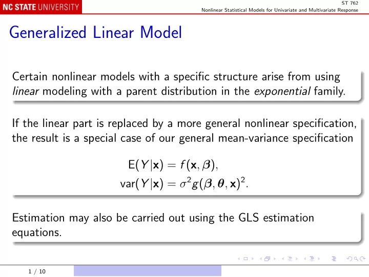
ST 762 Nonlinear Statistical Models for Univariate and Multivariate Response Generalized Linear Model Certain nonlinear models with a specific structure arise from using linear modeling with a parent distribution in the exponential family. If the linear part is replaced by a more general nonlinear specification, the result is a special case of our general mean-variance specification E( Y | x ) = f ( x , β ) , var( Y | x ) = σ 2 g ( β , θ , x ) 2 . Estimation may also be carried out using the GLS estimation equations. 1 / 10

ST 762 Nonlinear Statistical Models for Univariate and Multivariate Response The (Scaled) Exponential Family Y has a scaled exponential family distribution if its density (or probability mass function) is of the form � y ξ − b ( ξ ) � f ( y ; ξ, σ ) = exp + c ( y , σ ) . σ 2 ξ is the canonical parameter, and σ is the scale parameter. If σ 2 is known, this is the usual one-parameter exponential family with canonical parameter ξ . If σ 2 is unknown, it may or may not be the usual two-parameter exponential family. 2 / 10

ST 762 Nonlinear Statistical Models for Univariate and Multivariate Response Moments: E( Y ) = b ξ ( ξ ) = db ( ξ ) d ξ , var( Y ) = σ 2 b ξξ ( ξ ) = σ 2 d 2 b ( ξ ) d ξ 2 . If E( Y ) = µ = b ξ ( ξ ), then ξ = b − 1 ξ ( µ ). The function b − 1 ξ ( · ) is called the canonical link function , because it links the canonical parameter ξ to the mean µ . 3 / 10

ST 762 Nonlinear Statistical Models for Univariate and Multivariate Response Also var( Y ) = σ 2 b ξξ b − 1 = σ 2 g ( µ ) 2 , � � ξ ( µ ) so the variance depends on the mean in a specific way. Examples of the scaled exponential family: g ( µ ) 2 Distribution b ( ξ ) ξ ( µ ) Normal, σ 2 = 1 ξ 2 / 2 µ 1 Poisson exp( ξ ) log µ µ µ 2 Gamma − log( − ξ ) 1 /µ −√− 2 ξ 1 /µ 2 µ 3 Inverse Gaussian µ � 1 + e ξ � Binomial log log µ (1 − µ ) 1 − µ 4 / 10

ST 762 Nonlinear Statistical Models for Univariate and Multivariate Response Sufficiency If Y 1 , Y 2 , . . . , Y n is a random sample from a member of this family, the log-likelihood is n � Y j ξ − b ( ξ ) � � log L = + c ( Y j , σ ) σ 2 j =1 � � n n = 1 � � ξ Y j − nb ( ξ ) + c ( Y j , σ ) σ 2 j =1 j =1 so (if σ 2 is known) � Y j is sufficient for ξ . 5 / 10

ST 762 Nonlinear Statistical Models for Univariate and Multivariate Response Also, if Y 1 , Y 2 , . . . , Y n are independent, but in the distribution of Y j , ξ is replaced by ξ j = x T j β , the log-likelihood is   � T � n n n log L = 1 � � �  + β − b ( ξ j ) c ( Y j , σ ) Y j x j  σ 2 j =1 j =1 j =1 so now � Y j x j is sufficient for β . But note that � x T � E ( Y j | x j ) = µ j = b ξ ( ξ j ) = b ξ j β , so this is a conventional linear model only if b ξ ( ξ ) = ξ , i.e., for the normal distribution. Otherwise, it is a generalized linear model. 6 / 10

ST 762 Nonlinear Statistical Models for Univariate and Multivariate Response Note that b ξ ( · ) is determined by the distribution. We can replace it by a different function � x T � E ( Y j | x j ) = f j β , and it is still called a generalized linear model. Because the link f − 1 ( · ) is no longer the canonical link, we lose sufficiency–not a big deal. R and SAS support fitting these models with the link function chosen from a list. 7 / 10

ST 762 Nonlinear Statistical Models for Univariate and Multivariate Response Example: Six Cities Wheezing data Response: child wheezes at age 9 (0 or 1). Predictor: mother’s smoking status (0 = none, 1 = moderate, 2 = heavy). Possible covariate: community (Portage or Kingston). 8 / 10

ST 762 Nonlinear Statistical Models for Univariate and Multivariate Response Model: Y j ∼ Bernoulli ( µ j ) . Canonical link: � µ j � = x T log j β 1 − µ j or � x T � exp j β E ( Y j | x j ) = µ j = � � 1 + exp x T j β Logistic regression. � � x T Alternative link: probit function, µ j = Φ j β . 9 / 10

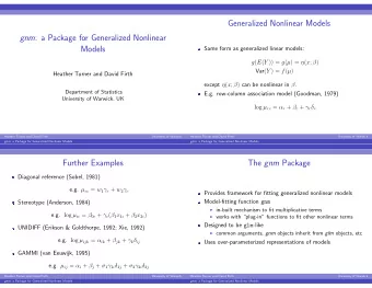
ST 762 Nonlinear Statistical Models for Univariate and Multivariate Response Generalized Nonlinear Model We may want a more general specification for the conditional mean: E ( Y j | x j ) = f ( x j , β ) . This is consistent with the scaled exponential family if ξ j satisfies b ξ ( ξ j ) = f ( x j , β ) . The mean-variance relationship is still determined by the distribution: var ( Y j | x j ) = σ 2 g { E ( Y j | x j ) } 2 = σ 2 g { f ( x j , β ) } 2 . 10 / 10