Bayesian Methods 1 Chris Williams School of Informatics, University - PowerPoint PPT Presentation
Bayesian Methods 1 Chris Williams School of Informatics, University of Edinburgh October 2015 1 / 23 Overview Introduction to Bayesian Statistics: Learning a Bernoulli probability Learning a discrete distribution Learning the mean
Bayesian Methods 1 Chris Williams School of Informatics, University of Edinburgh October 2015 1 / 23
Overview ◮ Introduction to Bayesian Statistics: Learning a Bernoulli probability ◮ Learning a discrete distribution ◮ Learning the mean of a Gaussian ◮ Exponential family ◮ Readings: Murphy § 3.3 (Beta), § 3.4 (Dirichlet), § 4.6.1 (Gaussian) Barber § 9.1.1, 9.1.3 (Beta), § 9.4.3 (no parents, Dirichlet), § 8.8.2 (Gaussian) 2 / 23
Bayesian vs Frequentist Inference Frequentist ◮ Assumes that there is an unknown but fixed parameter θ ◮ Estimates θ with some confidence ◮ Prediction by using the estimated parameter value Bayesian ◮ Represents uncertainty about the unknown parameter ◮ Uses probability to quantify this uncertainty. Unknown parameters as random variables ◮ Prediction follows rules of probability 3 / 23
Frequentist method ◮ Model p ( x | θ, M ) , data D = { x 1 , . . . , x N } ˆ θ = argmax θ p ( D | θ, M ) ◮ Prediction for x n +1 is based on p ( x n +1 | ˆ θ, M ) 4 / 23
Bayesian method ◮ Prior distribution p ( θ | M ) ◮ Posterior distribution p ( θ | D, M ) p ( θ | D, M ) = p ( D | θ, M ) p ( θ | M ) p ( D | M ) ◮ Making predictions � p ( x N +1 | D, M ) = p ( x N +1 , θ | D, M ) dθ � p ( x N +1 | θ, D, M ) p ( θ | D, M ) dθ = � p ( x N +1 | θ, M ) p ( θ | D, M ) dθ = Interpretation: average of predictions p ( x N +1 | θ, M ) weighted by p ( θ | D, M ) ◮ Marginal likelihood (important for model comparison) � p ( D | M ) = P ( D | θ, M ) P ( θ | M ) dθ 5 / 23
Bayes, MAP and Maximum Likelihood � p ( x N +1 | D, M ) = p ( x N +1 | θ, M ) p ( θ | D, M ) dθ ◮ Maximum a posteriori value of θ θ MAP = argmax θ p ( θ | D, M ) Note: not invariant to reparameterization (cf ML estimator); ex: variance and precision ( τ = 1 /σ 2 ) for a Gaussian ◮ If posterior is sharply peaked about the most probable value θ MAP then p ( x N +1 | D, M ) ≃ p ( x N +1 | θ MAP , M ) ◮ In the limit N → ∞ , θ MAP converges to ˆ θ (as long as p (ˆ θ ) � = 0 ) ◮ Bayesian approach most effective when data is limited, N is small 6 / 23
Learning probabilities: thumbtack example Frequentist Approach ◮ The probability of heads θ is unknown heads tails ◮ Given iid data, estimate θ using an estimator with good properties (e.g. ML estimator) 7 / 23
Likelihood ◮ Likelihood for a sequence of heads (1) and tails (0) p (1100 . . . 001 | θ ) = θ N 1 (1 − θ ) N 0 ◮ MLE N 1 ˆ θ = N 1 + N 0 8 / 23
Learning probabilities: thumbtack example Bayesian Approach: (a) the prior ◮ Prior density p ( θ ) , use Beta distribution p ( θ ) = Beta( α, β ) ∝ θ α − 1 (1 − θ ) β − 1 for α, β > 0 ◮ Properties of the Beta distribution � α E [ θ ] = θp ( θ ) = α + β αβ var( θ ) = ( α + β ) 2 ( α + β + 1) 9 / 23
Examples of the Beta distribution 3.5 2 1.8 3 1.6 1.4 2.5 1.2 2 1 0.8 1.5 0.6 0.4 1 0.2 0.5 0 0 0.1 0.2 0.3 0.4 0.5 0.6 0.7 0.8 0.9 1 0 0.1 0.2 0.3 0.4 0.5 0.6 0.7 0.8 0.9 1 Beta(0.5,0.5) Beta(1,1) 1.8 4.5 1.6 4 1.4 3.5 1.2 3 1 2.5 0.8 2 0.6 1.5 0.4 1 0.2 0.5 0 0 0 0.1 0.2 0.3 0.4 0.5 0.6 0.7 0.8 0.9 1 0 0.1 0.2 0.3 0.4 0.5 0.6 0.7 0.8 0.9 1 Beta(3,2) Beta(15,10) 10 / 23
Bayesian Approach: (b) the posterior p ( θ | D ) ∝ p ( θ ) p ( D | θ ) ∝ θ α − 1 (1 − θ ) β − 1 θ N 1 (1 − θ ) N 0 ∝ θ α + N 1 − 1 (1 − θ ) β + N 0 − 1 ◮ Posterior is also a Beta distribution ∼ Beta( α + N 1 , β + N 0 ) ◮ The Beta prior is conjugate to the binomial likelihood (i.e. prior and posterior have the same parametric form) ◮ α and β can be thought of as imaginary counts, with α + β as the equivalent sample size [cointoss demo] 11 / 23
Bayesian Approach: (c) making predictions � p ( X N +1 = heads | D, M ) = p ( X N +1 = heads | θ ) p ( θ | D, M ) dθ � = θ Beta( α + N 1 , β + N 0 ) dθ α + N 1 = α + β + N 12 / 23
Beyond Conjugate Priors ◮ The thumbtack came from a magic shop → a mixture prior p ( θ ) = 0 . 4Beta(20 , 0 . 5) + 0 . 2Beta(2 , 2) + 0 . 4Beta(0 . 5 , 20) 13 / 23
Generalization to multinomial variables ◮ Dirichlet prior r � θ α i − 1 p ( θ 1 , . . . , θ r ) = Dir( α 1 , . . . , α r ) ∝ i i =1 with � θ i = 1 , α i > 0 i ◮ α i ’s are imaginary counts, α = � i α i is equivalent sample size ◮ Properties E ( θ i ) = α i α ◮ Dirichlet distribution is conjugate to the multinomial likelihood 14 / 23
Examples of Dirichlet Distributions [Source: https://projects.csail.mit.edu/church/wiki/Models_with_Unbounded_Complexity] 15 / 23
◮ Likelihood r � θ N i ∝ i i =1 ◮ Show that MLE ˆ θ i = N i /N ◮ Posterior distribution r � θ α i + N i − 1 p ( θ | N 1 , . . . , N r ) ∝ i i =1 ◮ Marginal likelihood r Γ( α ) Γ( α i + N i ) � p ( D | M ) = Γ( α + N ) Γ( α i ) i =1 16 / 23
Inferring the mean of a Gaussian ◮ Likelihood p ( x | µ ) ∼ N ( µ, σ 2 ) ◮ Prior p ( µ ) ∼ N ( µ 0 , σ 2 0 ) ◮ Given data D = { x 1 , . . . , x N } , what is p ( µ | D ) ? 17 / 23
p ( µ | D ) ∼ N ( µ N , σ 2 N ) with N x = 1 � x n N i =1 Nσ 2 σ 2 0 µ N = 0 + σ 2 x + 0 + σ 2 µ 0 Nσ 2 Nσ 2 1 = N σ 2 + 1 σ 2 σ 2 N 0 ◮ See Murphy § 4.6.1 or Barber § 8.8.2 for details 18 / 23
The exponential family ◮ Any distribution over some x that can be written as η T u ( x ) � � P ( x | η ) = h ( x ) g ( η ) exp with h and g known, is in the exponential family of distributions. ◮ Many common distributions are in the exponential family. A notable exception is the t -distribution. ◮ The η are called the natural parameters of the distribution . ◮ For most distributions, the common representation (and parameterization) does not take the exponential family form. ◮ So sometimes useful to convert to exponential family representation and find the natural parameters. ◮ Exercise: Why not try this for some of the distributions that we’ve seen already! 19 / 23
Conjugate exponential models ◮ If the prior takes the same functional form as the posterior for a given likelihood, a prior is said to be conjugate for that likelihood ◮ There is a conjugate prior for any exponential family distribution ◮ If the prior and likelihood are conjugate and exponential, then the the model is said to be conjugate exponential ◮ In conjugate exponential models, the Bayesian integrals can be done analytically 20 / 23
Reflecting on Conjugacy ◮ All of the priors that we have seen so far are conjugate ◮ Good thing: easy to do the sums ◮ Bad thing: prior distribution should match beliefs. Does a Beta distribution match your beliefs? Is it good enough? ◮ Certainly not always ◮ Use of approximate inference methods for non-conjugate models (see later in MLPR) 21 / 23
Comparing Bayesian and Frequentist approaches ◮ Frequentist : fix θ , consider all possible data sets generated with θ fixed ◮ Bayesian : fix D , consider all possible values of θ ◮ One view is that Bayesian and Frequentist approaches have different definitions of what it means to be a good estimator 22 / 23
Summary of Bayesian Methods ◮ Maximum likelihood fails to capture prior or uncertainty ◮ Need to use a prior distribution (maximum likelihood equals MAP with uniform prior) ◮ Prior distribution might have its own parameters (usually called hyper-parameters) ◮ MAP fails to capture uncertainty, need full posterior distribution ◮ Prediction using MAP parameters does not capture uncertainty ◮ Do inference by marginalization. Inference and Learning are just using the rules of probability 23 / 23
Recommend
More recommend
Explore More Topics
Stay informed with curated content and fresh updates.


