Generalized Kitaev Spin-1/2 Models in Arbitrary Dimensions Yi Zhou - PowerPoint PPT Presentation
New F Front ntiers of S Strong ngly ly Co Correla lated M d Mat aterial als Exact Solution to a Class of Generalized Kitaev Spin-1/2 Models in Arbitrary Dimensions Yi Zhou Zhejiang University, Hangzhou Kavli ITS, Beijing, August 7 th
New F Front ntiers of S Strong ngly ly Co Correla lated M d Mat aterial als Exact Solution to a Class of Generalized Kitaev Spin-1/2 Models in Arbitrary Dimensions Yi Zhou Zhejiang University, Hangzhou Kavli ITS, Beijing, August 7 th , 2018
Collaborators Ji Jian-Jian Mia Miao Hui-Ke Hu Ke Jin Jin Fa a Wan ang Fu Fu-Chun Zh Zhang Kavli ITS Ka ITS Zhejiang Uni Zh Univ. Peking Un Univ. Ka Kavli ITS ITS References: [1] J. J. Miao, H. K. Jin, F. Wang, F. C. Zhang, YZ , arXiv:1806.06495 (2018). [2] J. J. Miao, H. K. Jin, F. C. Zhang, YZ , arXiv: 1806.10960 (2018).
Outline A brief introduction to Kitaev honeycomb model The construction of exactly solvable models Generating new models: 1D, 2D and 3D A particular example in 2D: a Mott insulator model 3D examples and possible realization in real materials
Kitaev Honeycomb model Spin-1/2 model (compass model) Kitaev (2006) Brick-wall representation Exact solvability Quantum paramagnet SU(2) invariant ground state Emergent SU(2) symmetry Fractional spin excitations Topologically distinct phases Feng, Zhang, Xiang (2007); Chen, Nussinov (2008) Two spins per unit cell
Existing generalizations Spin-1/2 models in 2D Yao, Kivelson (2007); Yang, Zhou, Sun (2007); Baskaran, Santhosh, Shankar (2009); Tikhonov, Feigelman (2010); Kells, Kailasvuori, Slingerland, Vala (2011); … Spin-1/2 models in 3D Si, Yu (2007); Ryu (2009); Mandal, Surendran (2009); Kimchi, Analytis, Vishwanath (2014); Nasu, Udagawa, Motome (2014); Hermanns, O'Brien, Trebst (2015); Hermanns, Trebst (2016); … Multiple-spin interactions Kitaev (2006); Lee, Zhang, Xiang (2007); Yu, Wang (2008); … SU(2)- invariant models F. Wang(2010); Yao, Lee (2011); Lai and O. I. Motrunich (2011); … Higher spin models Yao, Zhang, Kivelson (2009); Wu, Arovas, Hung (2009); Chern (2010); Chua, Yao, Fiete (2011); Nakai, Ryu, Furusaki (2012); Nussinov , van den Brink, (2013); …
Our goals Provide some generic rules for searching generalized Kitaev spin-1/2 models in arbitrary dimensions. Constrict ourselves on spin-1/2 models. Demonstrate some models of particular interest.
Construction of spin-1/2 models Basic idea: ① Construct exactly solvable 1D spin chains and ② then couple them to form a connected lattice in arbitrary dimensions. Steps: ① Construct spin-1/2 chains that can be exactly solved by the Jordan-Wigner transformation. ② Couple these chains to form a connected lattice on which the spin-1/2 model can be still exactly solved by the Jordan-Wigner transformation. Parquet rules: ① Elementary rules ② Supplementary rules
Sites and links on a lattice Consider a 𝒆 -dimensional cube, 𝒆 = 𝟑, 𝟒, 𝟓, ⋯ Site labelling: 𝒐 = 𝒐 𝟐 , 𝒐 𝟑 , ⋯ , 𝒐 𝒆 , 1 ≤ 𝒐 𝒌 ≤ 𝑴 𝒌 , 𝒌 = 1,⋯,𝒆 Ordering of sites 𝒌−𝟐 𝑴 𝒌 , for each site 𝒐; Define a number, 𝑶 = 𝒐 𝟐 + σ 𝒌=𝟑 𝒆 𝒐 𝒌 − 𝟐 ς 𝒎=𝟐 If 𝑶 < 𝑵, then 𝒐 < 𝒏. Link: a pair of sites (𝒐, 𝒏) 𝒆 Local link: σ 𝒌=𝟐 𝒐 𝒌 − 𝒏 𝒌 = 𝟐 𝒆 Nonlocal link: σ 𝒌=𝟐 𝒐 𝒌 − 𝒏 𝒌 > 𝟐 ordering of sites local and nonlocal links
Construction rules Model Hamiltonian (2) (2) (𝑁) 𝐼 = 𝐼 𝑚𝑝𝑑𝑏𝑚 + 𝐼 𝑜𝑝𝑜𝑚𝑝𝑑𝑏𝑚 + 𝐼 𝑜𝑝𝑜𝑚𝑝𝑑𝑏𝑚 Interactions (2) : local two−spin terms, 𝐾 𝑜,𝑜+ 𝛽𝛾 𝛾 𝑨𝑨 𝑨 𝛽 𝜏 𝑜+ 𝑨 𝜏 𝑜+ 𝐼 𝑚𝑝𝑑𝑏𝑚 𝜏 𝑜 and 𝐾 𝑜,𝑜+ 𝜏 𝑜 ; 𝑙 𝑙 1 1 𝑨𝑨 𝜏 𝑜 (2) 𝑨 ; 𝐼 𝑜𝑝𝑜𝑚𝑝𝑑𝑏𝑚 𝑨 𝜏 𝑛 : nonlocal two−spin terms, 𝐾 𝑜𝑛 𝑨 𝜏 𝑛 𝛽 ς 𝑜<𝑚<𝑛 𝜏 𝑚 (𝑁) 𝛽𝛾 𝜏 𝑜 𝛾 , etc., 𝐼 𝑜𝑝𝑜𝑚𝑝𝑑𝑏𝑚 : nonlocal multiple−spin terms, 𝐾 𝑜𝑛 where 𝛽, 𝛾 = 𝑦, 𝑧, and 𝑙 = 1, ⋯ , መ 𝑒 .
Construction rules Firstly, divide the lattice into white (w) and black (b) sublattices arbitrary. Elementary rules: 𝒚 𝝉 𝒏 𝒚 ① For a (local or nonlocal) link (𝑜, 𝑛) : 𝝉 𝒐 𝒚−bond 𝒛 𝝉 𝒏 𝒛 an 𝑦 -bond is allocated for 𝑜 ∈ 𝑥 and 𝑛 ∈ 𝑐 ; 𝝉 𝒐 𝒛−bond 𝒛 a 𝑧 -bond is allocated for 𝑜 ∈ 𝑐 and 𝑛 ∈ 𝑥 ; 𝒚 𝝉 𝒏 𝒚𝒛−bond 𝝉 𝒐 an 𝑦𝑧 -bond is allocated for 𝑜 ∈ 𝑥 and 𝑛 ∈ 𝑥 ; 𝒛 𝝉 𝒏 𝒚 𝝉 𝒐 𝒛𝒚−bond a 𝑧𝑦 -bond is allocated for 𝑜 ∈ 𝑐 and 𝑛 ∈ 𝑐 ; 𝒜 𝝉 𝒏 𝒜 𝝉 𝒐 𝒜−bond ② Different 𝑨 -bonds are not allowed to share the same site. beyond compass models
Construction rules Exactly solvability: quadratic fermion terms Jordan-Wigner transformation Majorana fermion representation 𝜷𝜸 𝝉 𝒐 𝒜 𝝉 𝒏 𝜷 ෑ 𝜸 𝑲 𝒐𝒏 𝝉 𝒎 𝒐<𝒎<𝒏 𝜷𝜸 𝜸 𝜷 𝝉 𝒐+ 𝑲 𝒐,𝒐+ 𝝉 𝒐 𝟐 𝟐 All the possible quadratic γ−fermion terms by J−W transformation.
Construction rules Exactly solvability: biquadratic fermion terms 𝑨𝑨 𝜏 𝑜 Majorana fermion representation 𝑨 𝜏 𝑛 𝑨 𝐾 𝑜𝑛 Static 𝒂 𝟑 gauge field Elementary rules: ① … ② Different 𝑨 -bonds are not allowed " − ": 𝑜 & 𝑛 ∈ the same sublattice to share the same site. " + ": 𝑜 & 𝑛 ∈ opposite sublattice 𝐸 𝑜𝑛 , The eigenstates can be divided into 𝐸 𝑜′𝑛′ = 0 , 𝐸 𝑜𝑛 , 𝐼 = 0 . 𝐸 𝑜𝑛 ∶ a set of good quantum #s different sectors according to 𝐸 𝑜𝑛 . In each sector, allowed spin terms are trasformed to quadratic γ−fermion 2 𝐸 𝑜𝑛 = 1 ⇒ 𝐸 𝑜𝑛 = ±1 terms.
Construction rules Majorana fermion representation Separation of degrees of freedom It is possible that some isolated 𝜃 𝑜 do not show up in 𝐼 𝜃 ⇒ local degeneracy To lift the local degeneracy: couple isolated 𝜽 𝒐 using nonlocal terms quadratic 𝜃−fermion terms quadratic 𝛿−fermion terms
Construction rules Duality 𝑥 ⟺ 𝑐 A similar duality relates topological trivial and non-trivial phases in interacting Kitaev chains. 𝛿 ⟺ 𝜃 J.J. Miao, H.K. Jin, F.C. Zhang, YZ (2017) A way to construct new models quadratic 𝜃−fermion terms quadratic 𝛿−fermion terms
Construction rules Shortcut multiple-spin interactions New multiple-spin interaction
Construction rules Supplementary rules: ① To add 𝜃 -fermion quadratic terms using a nonlocal link (𝑜, 𝑛) : 𝑜 and 𝑛 are not allowed to coincide with site connected by existing z-bonds in the original Hamiltonian constructed subjected to the two elementary rules. ② To add shortcut multiple-spin interactions: for a step along the 1 -direction, 𝛾 𝛽 𝜏 𝑚+ the two-spin term should be 𝜏 𝑚 with 𝛽, 𝛾 = 𝑦, 𝑧; for a step along the 1 𝑨 𝜏 𝑚+𝜀 𝑨 with 𝜀 ≠ other directions, the two-spin terms should be 𝜏 𝑚 1 , and there must exist a local 𝑨 -bond on this step in the original Hamiltonian. ③ In the above, the indices 𝛽 and 𝛾 should be chosen as follows: for 𝑚 ∈ 𝑥 and 𝑚 + 1 ∈ 𝑐 , (𝛽, 𝛾) = (𝑦, 𝑦) ; for 𝑚 ∈ 𝑐 and 𝑚 + 1 ∈ 𝑥 , (𝛽, 𝛾) = (𝑧, 𝑧) ; for 𝑚 ∈ 𝑥 and 𝑚 + 1 ∈ 𝑥 , (𝛽, 𝛾) = (𝑦, 𝑧) ; for 𝑚 ∈ 𝑐 and 𝑚 + 1 ∈ 𝑐 , (𝛽, 𝛾) = (𝑧, 𝑦) .
Generating new models: 1D examples Three parent models in 1D 𝑥 ⟺ 𝑐 (1) duality 𝛿 ⟺ 𝜃 Dual models in 1D 𝒚−bond 𝒛−bond 𝒚𝒛−bond 𝒛𝒚−bond 𝒜−bond
Generating new models: 1D examples Three parent models in 1D (2) split one site and insert a local bond Models with enlarged unit cell 𝒚−bond 𝒛−bond 𝒚𝒛−bond 𝒛𝒚−bond 𝒜−bond
Generating new models: 1D examples (3) erase bonds and add nonlocal bonds 𝒚−bond 𝒛−bond 𝒚𝒛−bond 𝒛𝒚−bond 𝒜−bond
Generating new models: from 1D to 2D Two parent models in 2D couple through 𝒜−bond 𝒚−bond 𝒛−bond 𝒚𝒛−bond 𝒛𝒚−bond 𝒜−bond
Generating new models: 2D examples Duality transformation can be performed along each chain independently. 𝒚−bond 𝒛−bond 𝒚𝒛−bond 𝒛𝒚−bond 𝒜−bond
Generating new models: 2D examples Split sites and insert nonlocal bonds 𝒚−bond 𝒛−bond 𝒚𝒛−bond 𝒛𝒚−bond 𝒜−bond
Generating new models: 3D examples Two parent models in 3D Three types of unit cells
2D example: a Mott insulator model 𝑰 𝟏 : two−spin interactions 𝑰 𝟐 : four−spin interactions → lift local degeneracy Elementary plaquette & Flux operator
2D example: a Mott insulator model Majorana representation Jordan-Wigner transformation Static Z 2 gauge field:
2D example: a Mott insulator model Separation of degrees of freedom Majorana representation Exact solvability: Given 𝑬 𝒔 = ±𝟐 → Both 𝑰 𝟏 and 𝑰 𝟐 are quadratic form . 𝑰 𝟏 : Absence of 𝜽 𝟒 → 𝟑 𝑴 𝒚 𝑴 𝒛 /𝟑 −fold degeneracy 𝑰 𝟐 : Lift the local degeneracy
Recommend
More recommend
Explore More Topics
Stay informed with curated content and fresh updates.
