Frequent Itemset Mining prof. dr Arno Siebes Algorithmic Data - PowerPoint PPT Presentation
Frequent Itemset Mining prof. dr Arno Siebes Algorithmic Data Analysis Group Department of Information and Computing Sciences Universiteit Utrecht Battling Size The previous time we saw that Big Data has a size problem And we ended by
Frequent Itemset Mining prof. dr Arno Siebes Algorithmic Data Analysis Group Department of Information and Computing Sciences Universiteit Utrecht
Battling Size The previous time we saw that Big Data ◮ has a size problem And we ended by noting that ◮ sampling may help us to battle that problem From now on, our one goal is ◮ to show how sampling helps in Frequent Itsemset Mining Why this context? ◮ Frequent pattern mining is an important topic in unsupervised data mining with many applications ◮ Moreover, there are good theoretical results ◮ and the theory is based on sampling for classification ◮ which is a basic problem in machine learning
Posh Food Ltd . You own an upmarket supermarket chain, selling mindbogglingly expensive food and drinks to customers with more money than sense ◮ and you wonder how you can wring even more money out of your customers You think it might be a good idea to suggest items that go well with what they already plan to buy. ◮ e.g., that a bottle of Krug Clos d’Ambonnay goes very well with the Iranian Almas Beluga Caviar they just selected. But, unfortunately, you are not as rich as your client` ele, so you actually don’t know ◮ so, you decide to look for patterns in your data ◮ sets of items – also known as itemsets – that your customers regularly buy together. You decide to mine your data for all frequent itemsets ◮ all sets of items that have been bought more then θ times in your chain.
Your First Idea You collect all transactions over the past year in your chain ◮ there turn out to be millions of them, a fact that makes you happy. Since you only sell expensive stuff ◮ nothing below a thousand or so; you do sell potatoes, but only ”La Bonnotte” you only have a few thousand different items for sale. Since, you want to know which sets of items sell well, ◮ you decide to list simply all sets of items ◮ and check whether or not they were sold together θ times or more. And this is a terrible idea! ◮ as you discover when you break off the computation after a week long run
Why is it Naive? A set with n elements has 2 n subsets ◮ 2 1000 ≈ 10 301 The universe is about 14 × 10 9 years old ◮ and a year has about 31 million seconds A modern CPU runs at about 5Ghz = 5 × 10 9 Hz ◮ which means that the universe is about 14 × 10 9 × 31 × 10 6 × 5 × 10 9 = 2 , 2 × 10 25 clockticks old So, if your database fits into the CPU cache ◮ and you can check one itemset per clocktick ◮ and you can parallelise the computation perfectly You would need ◮ 10 301 / (2 , 2 × 10 25 ) ≈ 5 × 10 275 computers that have been running in parallel since the big bang to finish about now! The number of elementary particles in the observable universe is, according to Wikipedia, about 10 97 ◮ excluding dark matter
A New Idea Feeling disappointed, you idly query your database. ◮ how many customers bought your favourite combination? ◮ Wagyu beef with that beautiful white Italian truffle accompanied by a bottle of Roman´ ee-Conti Grand Cru And to your surprise you find 0! You search for a reason ◮ plenty people buy Wagyu or white truffle or Roman´ ee-Conti – actually, they belong to your top sold items ◮ quite a few people buy Wagyu and Roman´ ee-Conti and the same holds for Wagyu and white truffle ◮ but no-one buys white truffle and Roman´ ee-Conti ◮ those Philistines prefer a Chateau P´ etrus with their truffle! ◮ on second thoughts: not a bad idea Clearly you cannot buy Wagyu and white truffle and Roman´ ee-Conti more often ◮ than you buy white truffle and Roman´ ee-Conti!
A Priori With this idea in mind, you implement the A Priori algorithm ◮ simple levelwise search ◮ you only check sets of n elements for which all subsets of n − 1 elements are frequent After you finished your implementation ◮ you throw your data at it ◮ and a minute or so later you have all your frequent itemsets. In principle, all subsets could be frequent ◮ and A Priori would be as useless as the naive idea But, fortunately, people do not buy that many different items in one transaction ◮ whatever you seem to observe on your weekly shopping run
Transaction Databases After this informal introduction, it is time to become more formal ◮ we have a set of items I = { i 1 , . . . , i n } ◮ representing, e.g., the items for sale in your store ◮ a transaction t is simply a subset of I , i.e., t ⊆ I ◮ or, more precisely, a pair ( tid , t ) in which tid ∈ N is the (unique) tuple id and t is a transaction in the sense above ◮ Note that there is no count of how many copies of i j the customer bought, just a record of the fact whether or not you bought i j ◮ you can easily represent that in the same scheme if you want ◮ A database D is a set of transactions ◮ all with a unique tid, of course ◮ if you don’t want to bother with tid’s, D is simply a bag of transactions
Frequent Itemsets Let D be a transaction database over I ◮ an itemset I is a set of items (duh), I ⊆ I ◮ itemset I occurs in transaction ( tid , t ) if I ⊆ t ◮ the support of an itemset in D is the number of transaction it occurs in supp D ( I ) = |{ ( tid , t ) ∈ D | I ⊆ t }| ◮ note that sometimes the relative form of support is used, i.e., supp D ( I ) = |{ ( tid , t ) ∈ D | I ⊆ t }| | D | ◮ An itemset I is called frequent if its support is equal or larger than some user defined minimal threshold θ I is frequent in D ⇔ supp D ( I ) ≥ θ
Frequent Itemset Mining The problem of frequent itemset mining is given by Given a transaction database D over a set of items I , find all itemsets that are frequent in D given the minimal support threshold θ . The original motivation for frequent itemset mining comes from association rule mining ◮ an association rule is given by a pair of disjoint itemsets X and Y ( X ∩ Y = ∅ ), it is denoted by X → Y ◮ where P ( XY ) ≥ θ 1 , is the (relative) support of the rule ◮ i.e., the relative supp D ( X ∪ Y ) = supp D ( XY ) ≥ θ 1 ◮ and P ( Y | X ) ≥ θ 2 is the confidence of the rule ◮ i.e., supp D ( XY ) supp D ( X ) ≥ θ 2
Association Rules The motivation of association rule mining is simply the observation that ◮ people that buy X also tend to buy Y ◮ for suitable thresholds θ 1 , θ 2 ◮ which may be valuable information for sales and discounts But then you might think ◮ correlation is no causation ◮ all you see is correlation And you are completely right ◮ but why would the supermarket manager care? ◮ if he sees that ice cream and swimming gear are positively correlated ◮ he knows that if sales of the one goes up, so will (likely) the sales of the other ◮ whether or not there is a causal relation or both are caused by an external factor like nice weather.
Discovering Association Rules Given that there are two thresholds, discovering association rules is usually a two step procedure ◮ first discover all frequent itemsets wrt θ 1 ◮ for each such frequent itemset I consider all partitions of I to check whether or not that partition satisfies the second condition ◮ actually one should be a bit careful so that you don’t consider partitions that cannot satisfy the second requirement ◮ which is very similar to the considerations in discovering the frequent itemsets The upshot is that the difficult part is ◮ discovering the frequent itemsets Hence, most of the algorithmic effort has been put ◮ in exactly that task Later on it transpired that frequent itemsets ◮ or, more general, frequent patterns have a more general use, we will come back to that, briefly, later
Discovering Frequent Itemsets Obviously, simply checking all possible itemsets to see whether or not they are frequent is not doable ◮ 2 |I| − 1 is rather big, even for small stores Fortunately, there is the A Priori property I 1 ⊆ I 2 ⇒ supp D ( I 1 ) ≥ supp D ( I 2 ) Proof { ( tid , t ) ∈ D | I 2 ⊆ t } = { ( tid , t ) ∈ D | I 1 ⊆ I 2 ⊆ t } ⊆ { ( tid , t ) ∈ D | I 1 ⊆ t } since I 1 ⊆ I 2 ⊆ t is a stronger requirement than I 1 ⊆ t . So, we have supp D ( I 2 ) = |{ ( tid , t ) ∈ D | I 2 ⊆ t }| ≤ |{ ( tid , t ) ∈ D | I 1 ⊆ t }| = supp D ( I 1 ) If I 1 is not frequent in D , neither is I 2
Levelwise Search Hence, we know that: if Y ⊆ X and supp D ( X ) ≥ t 1 , then supp D ( Y ) ≥ t 1 . and conversely, if Y ⊆ X and supp D ( Y ) < t 1 , then supp D ( X ) < t 1 . In other words, we can search levelwise for the frequent sets. The level is the number of items in the set: A set X is a candidate frequent set iff all its subsets are frequent. Denote by C ( k ) the sets of k items that are potentially frequent (the candidate sets) and by F ( k ) the frequent sets of k items.
Apriori Pseudocode Algorithm 1 Apriori( θ , I , D ) 1: C (1) ← I 2: k ← 1 3: while C ( k ) � = ∅ do F ( k ) ← ∅ 4: for all X ∈ C ( k ) do 5: if supp D ( X ) ≥ θ then 6: F ( k ) ← F ( k ) ∪ { X } 7: end if 8: end for 9: C ( k + 1) ← ∅ 10: for all X ∈ F ( k ) do 11: for all Y ∈ F ( k ) that share k − 1 items with X do 12: if All Z ⊂ X ∪ Y of k items are frequent then 13: C ( k + 1) ← C ( k + 1) ∪ { X ∪ Y } 14: end if 15: end for 16: end for 17: k ← k + 1 18: 19: end while
Example: the data tid Items 1 ABE 2 BD 3 BC 4 ABD 5 AC 6 BC 7 AC 8 ABCE 9 ABC Minimum support = 2
Example: Level 1 tid Items 1 ABE 2 BD Candidate Support Frequent? 3 BC A 6 Yes 4 ABD B 7 Yes 5 AC C 6 Yes 6 BC D 2 Yes 7 AC E 2 Yes 8 ABCE 9 ABC
Recommend
More recommend
Explore More Topics
Stay informed with curated content and fresh updates.
