Frequent Subgraph Mining Frequent Subgraph Mining (FSM) Outline FSM - PowerPoint PPT Presentation
Frequent Subgraph Mining Frequent Subgraph Mining (FSM) Outline FSM Preliminaries FSM Algorithms gSpan complete FSM on labeled graphs SUBDUE approximate FSM on labeled graphs SLEUTH FSM on trees Review FSM In
Frequent Subgraph Mining
Frequent Subgraph Mining (FSM) Outline • FSM Preliminaries • FSM Algorithms – gSpan – complete FSM on labeled graphs – SUBDUE – approximate FSM on labeled graphs – SLEUTH – FSM on trees • Review
FSM In a Nutshell • Discovery of graph structures that occur a significant number of times across a set of graphs • Ex.: Common occurrences of hydroxide-ion • Other instances: – Finding common biological pathways among species. – Recurring patterns of humans interaction during an epidemic. Carbonic Acid – Highlighting similar data to reveal data set as a whole. H O H Sulfuric Acid Acetic Acid O O O C O H O S H C C Ammonia O O H H O H H H H N H
FSM Preliminaries • Support is some integer or frequency • Frequent graphs occur more than support number of times. O-H present in ¾ inputs � frequent if support <= 3 Carbonic Acid H O H Sulfuric Acid Acetic Acid O O O C O H O S H C C Ammonia O O H H O H H H H N H
What Makes FSM So Hard? • Isomorphic graphs have same structural properties even though they may look different. • Subgraph isomorphism problem : Does a graph contain a subgraph isomorphic to another graph? • FSM algorithms encounter this problem while buildings graphs. • This problem is known to be NP-complete ! A B A B Isomorphic under A,B,C,D labeling C D D C
Pattern Growth Approach • Underlying strategy of both traditional frequent pattern mining and frequent subgraph mining • General Process: – candidate generation : which patterns will be considered? For FSM, – candidate pruning : if a candidate is not a viable frequent pattern, can we exploit the pattern to prevent unnecessary work? • subgraphs and subsets exponentiate as size increases! – support counting : how many of a given pattern exist? • These algorithms work in a breadth-first or depth-first way. – Joins smaller frequent sets into larger ones. – Checks the frequency of larger sets.
Pattern Growth Approach – Apriori • Apriori principle: if an itemset is frequent, then all of its subsets are also frequent. – Ex. if itemset {A, B, C, D} is frequent, then {A, B} is frequent. – Simple proof: With respect to frequency, all sets trivially contain their subsets, thus frequency of subset >= frequency of set. – Same property applies to (sub)graphs! • Apriori algorithm exploits this to prune huge sections of the search space! ∅ If A is infrequent, no A B C supersets with A can be frequent! AB AC BC ABC
FSM Algorithms Discussed • gSpan – complete frequent subgraph mining – improves performance over straightforward apriori extensions to graphs through DFS Code representation and aggressive candidate pruning • SUBDUE – approximate frequent subgraph mining – uses graph compression as metric for determining a “frequently occuring” subgraph • SLEUTH – complete frequent subgraph mining – built specifically for trees
FSM – R package • R package for FSM is called subgraphMining • To import: install.packages(“subgraphMining”) • Package contains: gSpan, SUBDUE, SLUETH. • Also contains the following data sets: – cslogs – metabolicInteractions. • To load the data, use the following code: # The cslogs data set data(cslogs) # The matabolicInteractions data data(metabolicInteractions)
FSM Outline • FSM Preliminaries • FSM Algorithms – gSpan – SUBDUE – SLEUTH • Review
gSpan: Graph-Based Substructure Pattern Mining • Written by Xifeng Yan & Jiawei Han in 2002. • Form of pattern-growth mining algorithm. – Adds edges to candidate subgraph – Also known as, edge extension • Avoid cost intensive problems like – Redundant candidate generation – Isomorphism testing • Uses two main concepts to find frequent subgraphs – DFS lexicographic order – minimum DFS code
gSpan Inputs • Set of graphs, support • Graph of form � = ( � , � , � � , � � ) – � , � – vertex and edge sets – � � – vertex labels – � � – edge labels – label sets need not be one-to-one H O H � � = { � , � , � } � � = { single−bond, double−bond } O C O
gSpan Components Strategy: • build frequent subgraphs bottom-up , using DFS code as regularized representation • eliminate redundancies via minimal DFS codes based on code lexicographic ordering Depth-first Search (DFS) Code structured graph representation for building, comparing DFS Lexicographic minimal DFS code Order selection, pruning of canonical comparison subgraphs of graphs
Depth First Search Primer Todo…?
gSpan: DFS codes Code Edge # DFS Code: sequence of edges traversed during DFS 0 (0,1,X,a,Y) 1 (1,2,Y,b,X) Vertex discovery 2 (2,0,X,a,X) times 3 (2,3,X,c,Z) 0 X 4 (3,1,Z,b,Y) 5 (1,4,Y,d,Z) a a 1 Y d Format: ( � , � , � � , � ( � , � ) , � � ) 4 b Z � , � – vertices by time of discovery b X 2 � � , � � - vertex labels of � � , � � c � ( � , � ) – edge label between � � , � � 3 Z � < � : forward edge � > � : back edge
DFS Code: Edge Ordering • Edges in code ordered in very specific manner, corresponding to DFS process • � � = ( � � , � � ), � � = ( � � , � � ) • � � ≺ � � � � � appears before � � in code • Ordering rules: 1. if � � = � � and � � < � � � � � ≺ � � • from same source vertex, � � traversed before � � in DFS 2. if � � < � � and � � = � � � � � ≺ � � • � � is a forward edge and � � traversed as result of � � traversal if � � ≺ � � and � � ≺ � � , � � � ≺ � � 3. • ordering is transitive
DFS Code: Edge Ordering Example 0 Code Edge # X • Rule applications by edge # a a 0 (0,1,X,a,Y) • 0 ≺ 1 (Rule 2) 1 Y 1 (1,2,Y,b,X) d • 1 ≺ 2 (Rule 2) 2 (2,0,X,a,X) 4 b Z • 0 ≺ 2 (Rule 3) 3 (2,3,X,c,Z) b 2 X 4 (3,1,Z,b,Y) • 2 ≺ 3 (Rule 1) 5 (1,4,Y,d,Z) c • Exercise: what 3 Z others? Edge ordering can be recorded easily during the DFS!
Graphs have multiple DFS Codes! Exercise: Write the 2 rightmost graphs using DFS code 0 0 0 X Y X X d 4 b a a a a a a Z 1 1 X 1 X Y Y b d d 4 a a b b Z Z c b b b Y 2 X 2 X 2 X d b c c c Z 3 3 3 Z Z Z Z 4 solution to redundant DFS codes: lexical ordering, minimal code!
DFS Lexicographic Ordering vs. DFS Code • DFS code: Ordering of edge sequence of a particular DFS – E.g. DFS’s that start at different vertices may have different DFS codes • Lexicographic ordering: ordering between different DFS codes
DFS Lexicographic Ordering • Given lexicographic ordering of label set � , ≺ � • Given graphs � � , � � (equivalent label sets). • Given DFS codes – � = code � � , � � = � � , � � , … , � � – � = code � � , � � = � � , � � , … , � � – (assume � ≥ � ) • � ≤ � iff either of the following are true: – ∃ � , 0 ≤ � ≤ min � , � such that • � � = � � for � < � and • � � ≺ � � � – � � = � � ��� 0 ≤ � ≤ �
DFS Lex. Ordering: Edge Comparison • Given DFS codes – � = code � � , � � = � � , � � , … , � � – � = code � � , � � = � � , � � , … , � � – (assume � ≥ � ) • Given � such that � � = � � for � < � • Given � � = � � , � � , � � � , � � � , � � , � � � , � � = � � , � � , � � � , � � � , � � , � � � , • � � ≺ � � � if one of the following cases Case 1 : Both forward edges, AND… Case 3 : � � back , � � forward � � � ≺ � � � Case 2 : Both back edges, AND…
Edge Comparison: Case 1 (both forward) • Both forward edges, AND one of the following: – � � < � � (edge starts from a later visited vertex) • Why is this (think about DFS process)? – � � = � � AND labels of � lexicographically less than labels of � , in order of tuple. • Ex: Labels are strings, � � = __, __, m, e, x , � � = (__, __, m, u, x) – m = m, e < u � � � ≺ � � � • Note: if both forward edges, then � � = � � – Reasoning: all previous edges equal, target vertex discovery times are the same
Edge Comparison: Case 2 (both back) • Both back edges, AND one of the following: – � � < � � (edge refers to earlier vertex) – � � = � � AND edge label of � lexicographically less than � • Note: given that all previous edges equal, vertex labels must also be equal • Note: if both back edges, then � � = � � – Reasoning: all previous edges equal, source vertex discovery times are the same.
Code (A) Code (B) Code (C) Edge # 0 (0,1,X,a,Y) (0,1,Y,a,X) (0,1,X,a,X) 1 (1,2,Y,b,X) (1,2,X,a,X) (1,2,X,a,Y) 2 (2,0,X,a,X) (2,0,X,b,Y) (2,0,Y,b,X) 3 (2,3,X,c,Z) (2,3,X,c,Z) (2,3,Y,b,Z) 4 (3,1,Z,b,Y) (3,1,Z,b,X) (3,0,Z,c,X) 5 (1,4,Y,d,Z) (0,4,Y,d,Z) (2,4,Y,d,Z) 0 0 0 X X Y d a 4 a b a a Z 1 1 Y 1 X X d b 4 b a a Z b b c X 2 X 2 Y 2 d c c b Z 3 3 3 Z Z Z 4
Recommend
More recommend
Explore More Topics
Stay informed with curated content and fresh updates.
