Frank Kurth University of Bonn Proceedings of the Second - PowerPoint PPT Presentation

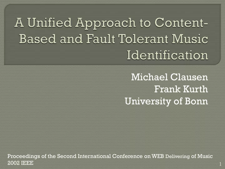
Michael Clausen Frank Kurth University of Bonn Proceedings of the Second International Conference on WEB Delivering of Music 2002 IEEE 1

Andreas Ribbrock Frank Kurth University of Bonn 2

 Introduction  Data Modeling  Fault Tolerance  Content-based Search in Scores  Content-based Search in Audio Data  Our Project  Article critics 3

 The two articles deal with indexing and searching of polyphonic and PCM audio  When dealing with polyphonic audio searching is done using pitches  When searching in PCM audio some massive data reduction needs to be done  Searching in PCM audio is accomplished by creating feature extractors 4

 Much related work use string-based representation  U represent all possible objects and D is a document D  U  Polyphonic music is represented by    : U P  Where Z is onset time, and P is the set of admissible pitches 5

   A query is a set of notes Q Z P Q  and a query is represented: {[ , ],....., [ , ]} t p t n p 1 1 n D   A hit on a query Q in a database ( ,...., ) D D 1 N        is a pair such that ( , ) [ 1 : ] t i Z N : { [ , ],..., [ , ]} Q t t t p t t p D 1 1 n n i  All exact hits are given by    ( ) : {( , ) | } H Q t i Q t D D i 6

F[x](n)   When modeling PCM audio we use a feature extractor   For a fixed feature extractor F and signal x we obtain a document consisting of all nonzero features along with there positions         D f (x) : {[n, ] | F[x](n) 0} [1 : c]  The set of all hits is defined by:    H (Q) : {(t, i) | D (Q) t D (x )} D F F F i 7

 In real scenarios users may not remember nodes are so some fault tolerance is needed  Two ways to deal with Fault Tolerance • k-Mismatches • Fuzzy Search 8

 k-mismatches is defined by which is all the matches to a ( ) H , Q D k query Q containing at most k non matching objects       {( , ) | ' , | ' | | | ' } t i Q Q Q Q k such that Q t D i  This can be used to create a ranked list if the output of is ( ) H , Q D k sorted in decreasing order 9

 Fuzzy search is used when there is doubt about certain parts of the query q   For each there is a set of alternatives and is called a Q q  F U fuzzy query . If there is no doubt about a specific q  one Q F Q would choose q  { q } F  An elementary query of is if there for each exist exactly q  F Q Q one alternative.  The hit of the fuzzy query is then<   {( , ) | } t j P t D for an elementary query P of F j Q 10

Example of a search Document D1with two queries   Q : {[0, 74], [4, 70]}, Q : {[4, 74], [8, 70]} 1 2 D1 := {[8, 74] , [11, 77], [11, 69], [12, 77], [12, 72], [16, 74], [16, 65], [20, 70], [23, 74], [23, 66],  [24, 74], [24, 69], [28, 70], [28, 62]} U     Then the set of all t such that is for is Q t D and Q t D 1 1 2 1   {( 16 , 1 ), ( 24 , 1 )} {(12, 1), (20, 1)} Q and Q 1 2 11

 If we include knowledge of metrical position we can reduce the exact hit of our queries  Our Universe is modified and takes nodes from the set  3 16    br      V : Z [0 : - 1 ] P     H ([0, , p]) : {(t, i) | [t, , p] D }   : 12 D i 4 u  Our Document transforms to D1 := {[0,8, 74] , [0,11, 77], [0,11, 69], [1,0, 77], [1,0, 72], [1,4, 74], [1,4, 65], [1,8, 70], [1,11, 74], [1,11, 66],  [2,0, 74], [2,0, 69], [2,4, 70], [2,4, 62]} U  The queries transform to   Q {[0, 0, 74], [0, 4, 70]} and Q { [0, 4, 74], [0, 8, 70]} 1 2  For the exact hit is (2,1) and for the exact hit is (1,1) Q Q 2 1 12

 MIDI database with 12000 songs and 327 MB in size.   Search index consist of the sets ([ 0 , , ) H D p  Hardware is Pentium II, 333 MHz, 256 MB RAM, Windows NT 4.0  Row a - Number of nodes in a query  Row b - Total system response  Row c - Time to fetch inverted lists 13

 The whistled song from a user normally have a different tempo than the original  The whistled tempo curve changes over time so rather than static s-times value, the changes lie between   s s s  u  The user whistles a song to an algorithm which outputs a sequence of MIDI-notes which can be edited in a program  A search for “Yellow Submarine” in the database with a rhythm tolerance of 10% 23 were found 14

15

 The audentify System is designed identify short excerpts (1-5 sek)  It takes use of feature extractors for a given base signal x ( x ) D F and a feature extractor F k    Feature density of a feature extractor is defined as if each n interval of length n taken from contains k features [ X ] F 16

 First a input signal is prefiltered, with a FIR filter f   [ ] : C f x f x denotes m-significant local maxima of x [ x ] M m  ' denotes local maxima on non-zero elements of x [ ] M m x    Then a operator is defined as a sequence that contains at the position of each significant maximum, the distance to the next significant maximum Q  Then a linear quantizer reduces the extracted distances to c c feature classes   '    F Q M C Max C K f 17

 A more robust Feature Extractor than the one showed before is based on the volume of the signal  First volume for a given signal is analyzed using Hamming- window  Then the smoothed by a low pass filter  The local maxima and minima is extracted using operator ' ' M K  Then the difference between the local maxima is found   ' ' ' :    F M C V , , Vol O O K f s w 1 2 18

 Both and are feature extractors which are working in the F F Max Vol time domain where the WFT-Feature is extracted from the frequency domain  A signal x is transformed into the frequency domain using a windowed Fourier transform  Then using an operator S the frequency centroid is calculated  Then a low pass filter is used, the local maxima are extracted and the distance is between the two consecutive local maxima are calculated        : F Q M C S w , wft c K f g s 19

 A problem with the feature extractors presented before is that two signals with different signal quality can different features  To solve this problem a rough binary quantizer is used on the signal  Then a string over a finite alphabet approximating the signal x is then produced using code. Two signals with different signal quality should then have the same string  Then the nearest codebook entry is denoted to a bit vector   C   : [ ] F C P x , code C n m 20

5 types of query signals is considered  Short parts of a track taken (cropped) from an arbitrary position within the track  MP3 re – encoded and decoded versions of a track were MP3 – compression is performed at 96 kbps  Tracks recorded by placing microphone in front of a loudspeaker  Tracks recorded by placing a cellular phone (GSM) in front of a loudspeaker 21

 Tracks recorded by a cellular phone with the incomming audio signal recorded by placing a microphone in front of the loudspeaker of a receiving phone  For signals 1-3 only a very short sample was needed to find a match. For signal 4-5 at least a sample of 15-20 seconds is needed before a match could be found 22

In our project we try to recognize PCM audio recorded from a mobile phone. We can use the knowledge about the different feature extractors and which ones are good to use when working with highly distored audio material 23

o Positive: o Many things from the two articles are relevant for our project o First half of the first article is easy to understand o Negative: o Requires some background knowledge to fully understand what is going on o Could use more examples and illustrations, there is a lot of text o Last half of the first article is hard to understand o The second article is very short and compressed 24