Foundations of pred(n) = set of all immediate predecessors of n p - PowerPoint PPT Presentation
Terminology: Program Representation e o ogy: og a ep ese tat o Control Flow Graph: Control Flow Graph: Nodes N statements of program Edges E flow of control Foundations of pred(n) = set of all immediate predecessors of
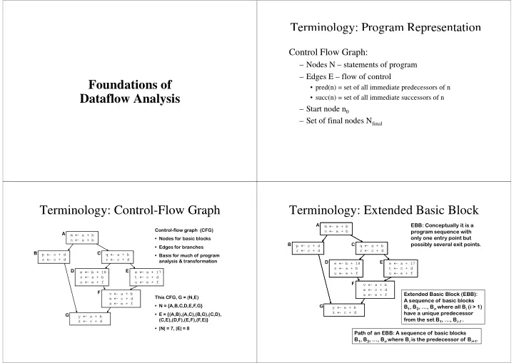
Terminology: Program Representation e o ogy: og a ep ese tat o Control Flow Graph: Control Flow Graph: – Nodes N – statements of program – Edges E – flow of control Foundations of • pred(n) = set of all immediate predecessors of n p ( ) p Dataflow Analysis • succ(n) = set of all immediate successors of n – Start node n 0 Start node n 0 – Set of final nodes N final Terminology: Control-Flow Graph Terminology: Control Flow Graph Terminology: Extended Basic Block Terminology: Extended Basic Block A EBB: Conceptually it is a m ← a + b Control-flow graph (CFG) g p ( ) n ← a + b n ← a b program sequence with program sequence with A A m ← a + b only one entry point but • Nodes for basic blocks n ← a + b possibly several exit points. B C p ← c + d q ← a + b • Edges for branches r ← c + d r ← c + d B B C C p ← c + d q ← a + b • Basis for much of program r ← c + d r ← c + d analysis & transformation D E e ← b + 18 e ← a + 17 s ← a + b t ← c + d D D E E e ← b + 18 e ← b + 18 e ← a + 17 e ← a + 17 u ← e + f u ← e + f f f s ← a + b t ← c + d u ← e + f u ← e + f F v ← a + b w ← c + d F F v ← a + b Extended Basic Block (EBB): x ← e + f This CFG, G = (N,E) w ← c + d A sequence of basic blocks x ← e + f • N = {A,B,C,D,E,F,G} G B 1 , B 2 , …, B n where all B i (i > 1) y ← a + b z ← c + d ← have a unique predecessor h i d • E = {(A,B),(A,C),(B,G),(C,D), + d G y ← a + b from the set B 1 , …, B i-1 . (C,E),(D,F),(E,F),(F,E)} z ← c + d • |N| = 7, |E| = 8 P th f Path of an EBB: A sequence of basic blocks EBB A f b i bl k B 1 , B 2 , …, B n where B i is the predecessor of B i+1 .
Terminology: Program Points Terminology: Program Points Dataflow Analysis Dataflow Analysis • One program point before each node • One program point before each node Compile-Time Reasoning About Compile Time Reasoning About • One program point after each node Run-Time Values of Variables or Expressions at Different Program Points • Join point – program point with multiple – Which assignment statements produced the value of Which assignment statements produced the value of predecessors predecessors the variables at this point? • Split point – program point with multiple – Which variables contain values that are no longer Which variables contain values that are no longer successors used after this program point? – What is the range of possible values of a variable at Wh i h f ibl l f i bl this program point? Dataflow Analysis: Basic Idea Dataflow Analysis: Basic Idea Forward Dataflow Analysis Forward Dataflow Analysis • Analysis propagates values forward through • Analysis propagates values forward through • Information about a program represented using • Information about a program represented using control flow graph with flow of control values from an algebraic structure called lattice – Each node has a transfer function f E h d h t f f ti f • Analysis produces a lattice value for each • Input – value at program point before node program point program point • Output – new value at program point after node O t t l t i t ft d • Two flavors of analyses – Values flow from program points after predecessor nodes to program points before successor nodes nodes to program points before successor nodes – Forward dataflow analyses – At join points, values are combined using a merge – Backward dataflow analyses f y function function • Canonical Example: Reaching Definitions
Backward Dataflow Analysis Backward Dataflow Analysis Partial Orders Partial Orders • Analysis propagates values backward through • Analysis propagates values backward through • Set P • Set P control flow graph against flow of control • Partial order ≤ such that ∀ x,y,z ∈ P – Each node has a transfer function f – x ≤ x (reflexive) • Input – value at program point after node – x ≤ y and y ≤ x implies x = y – x ≤ y and y ≤ x implies x = y (asymmetric) (asymmetric) • Output – new value at program point before node – x ≤ y and y ≤ z implies x ≤ z (transitive) – Values flow from program points before successor Values flow from program points before successor nodes to program points after predecessor nodes – At split points, values are combined using a merge – At split points values are combined using a merge function – Canonical Example : Live Variables C i l E l Li V i bl Upper Bounds Upper Bounds Lower Bounds Lower Bounds • If S ⊆ P then • If S ⊆ P then • If S ⊆ P then • If S ⊆ P then – x ∈ P is an upper bound of S if ∀ y ∈ S, y ≤ x – x ∈ P is a lower bound of S if ∀ y ∈ S, x ≤ y – x ∈ P is the least upper bound of S if – x ∈ P is the greatest lower bound of S if • x is an upper bound of S, and pp • x is a lower bound of S, and • x ≤ y for all upper bounds y of S • y ≤ x for all lower bounds y of S – ∨ - join , least upper bound (lub), supremum (sup) ∨ – ∧ – ∧ - meet , greatest lower bound (glb), infimum (inf) join , least upper bound (lub), supremum (sup) meet greatest lower bound (glb) infimum (inf) • ∨ S is the least upper bound of S • ∧ S is the greatest lower bound of S • x ∨ y is the least upper bound of {x y} x ∨ y is the least upper bound of {x,y} • x ∧ y is the greatest lower bound of {x y} • x ∧ y is the greatest lower bound of {x,y}
Coverings Coverings Example Example • Notation: x < y if x ≤ y and x ≠ y • Notation: x < y if x ≤ y and x ≠ y • P {000, 001, 010, 011, 100, 101, 110, 111} • P = {000 001 010 011 100 101 110 111} (standard boolean lattice, also called hypercube) • x ≤ y if (x bitwise and y) = x • x ≤ y if (x bitwise_and y) = x • x is covered by y (y covers x) if We can visualize a partial We can visualize a partial – x < y, and x < y and 111 order with a Hasse Diagram – x ≤ z < y implies x = z • If y covers x f 011 110 101 • Line from y to x Line from y to x • Conceptually, y covers x if there are no • Conceptually y covers x if there are no 010 • y is above x in diagram elements between x and y 001 100 000 Lattices Lattices Top and Bottom Top and Bottom • If x ∧ y and x ∨ y exist (i e are in P) for all x y ∈ P • If x ∧ y and x ∨ y exist (i.e., are in P) for all x,y ∈ P, • Greatest element of P (if it exists) is top ( T ) • Greatest element of P (if it exists) is top ( T ) then P is a lattice . • Least element of P (if it exists) is bottom ( ⊥ ) • If ∧ S and ∨ S exist for all S ⊆ P, If S d S i t f ll S P then P is a complete lattice . • Theorem: All finite lattices are complete • Example of a lattice that is not complete p p – Integers Z – For any x, y ∈ Z, x ∨ y = max(x,y), x ∧ y = min(x,y) y , y , y ( ,y), y ( ,y) – But ∨ Z and ∧ Z do not exist – Z ∪ { +∞ , −∞ } is a complete lattice { , } p
Connection between ≤ , ∧ , and ∨ Connection between ≤ ∧ and ∨ Connecting Lemma Proofs (1) Connecting Lemma Proofs (1) The following 3 properties are equivalent: • Proof of x ≤ y implies x ∨ y = y • Proof of x ≤ y implies x ∨ y y – x ≤ y – x ≤ y implies y is an upper bound of {x,y}. – x ∨ y = y – Any upper bound z of {x,y} must satisfy y ≤ z. – x ∧ y = x – So y is least upper bound of {x,y} and x ∨ y = y So y is least upper bound of {x,y} and x ∨ y • Will prove: Will prove: y – x ≤ y implies x ∨ y = y and x ∧ y = x • Proof of x ≤ y implies x ∧ y = x – x ∨ y = y implies x ≤ y x ∨ y y implies x ≤ y – x ≤ y implies x is a lower bound of {x,y}. i li i l b d f { } – x ∧ y = x implies x ≤ y – Any lower bound z of {x,y} must satisfy z ≤ x. • By Transitivity, • By Transitivity – So x is greatest lower bound of {x,y} and x ∧ y = x – x ∨ y = y implies x ∧ y = x – x ∧ y = x implies x ∨ y = y i li Connecting Lemma Proofs (2) Connecting Lemma Proofs (2) Lattices as Algebraic Structures Lattices as Algebraic Structures • Proof of x ∨ y • Proof of x ∨ y = y implies x ≤ y y implies x ≤ y • Have defined ∨ and ∧ in terms of ≤ • Have defined ∨ and ∧ in terms of ≤ – y is an upper bound of {x,y} implies x ≤ y • Will now define ≤ in terms of ∨ and ∧ • Proof of x ∧ y = x implies x ≤ y – Start with ∨ and ∧ as arbitrary algebraic operations – x is a lower bound of {x,y} implies x ≤ y – x is a lower bound of {x y} implies x ≤ y that satisfy associative, commutative, idempotence, y , , p , and absorption laws – Will define ≤ using ∨ and ∧ Will define ≤ using ∨ and ∧ – Will show that ≤ is a partial order
Recommend
More recommend
Explore More Topics
Stay informed with curated content and fresh updates.
